Rows: 2323000 Columns: 1
── Column specification ────────────────────────────────────────────────────────
Delimiter: ","
dbl (1): upload_day

ℹ Use `spec()` to retrieve the full column specification for this data.
ℹ Specify the column types or set `show_col_types = FALSE` to quiet this message.
this creates a new object called gp_freq_dist that contains each value within ice_tib but with an extra column/variable called days_group that indicates the bin the value of upload_day is in
NoteSet notation
the value of upload_day now has a corresponding value of days_group containing the bin
the first score of 34 has been assigned to the bin labelled `(30, 34] which is the bin containing any score above 30, up to and including 34
the label uses standard mathematical notation for sets where ( or ) means ‘not including’ and [ or ] means ‘including’
now we can use summarize() and n() to count scores like before, except to use days_group instead of upload_day
Coding challenge
Create a grouped frequency table called gp_freq_dist by starting with the code in the code example and then using the code we used to create freq_tbl to create a pipe that summarizes the grouped scores.
Show the code
gp_freq_dist<-ice_tib|>dplyr::mutate( days_group =ggplot2::cut_width(upload_day, 4))|>dplyr::group_by(days_group)|>dplyr::summarise( frequency =n())gp_freq_dist
we have an object gp_freq_dist that contains the number of days grouped into bins of 4 days and the number of videos uploaded during each of the time periods represented by those bins
to calculate the relative frequency we can use dplyr::mutate() to add a variable that divides the frequency by the total number of videos using sum()
... |>
    dplyr::mutate(
        relative_freq = frequency/sum(frequency) # creates a new column
    )
Efficient Code
rather than creating the table of relative frequencies step-by-step, it is usually more efficient to carry out the steps in one piece of code
Show the code
gp_freq_dist<-ice_tib|>dplyr::mutate( days_group =ggplot2::cut_width(upload_day, 4))|>dplyr::group_by(days_group)|>dplyr::summarise( frequency =n())|>dplyr::mutate( relative_freq =frequency/sum(frequency), percent =relative_freq*100)gp_freq_dist
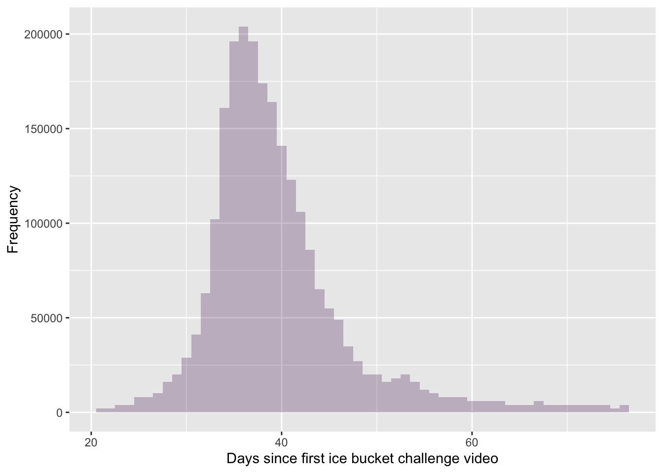
We’ve discussed elsewhere that if you include packages when you use functions (e.g., dplyr::mutate()) you don’t need to explicitly load the package (in this case dplyr). However, to create plots with ggplot2 you build them up layer by layer, which means you use a lot of ggplot2 functions. For this reason, I advise loading it at the start of your Quarto document and not worrying too much about including package references when you use functions. You can load it either with library(ggplot2) or by loading the entire tidyverse using library(tidyverse).
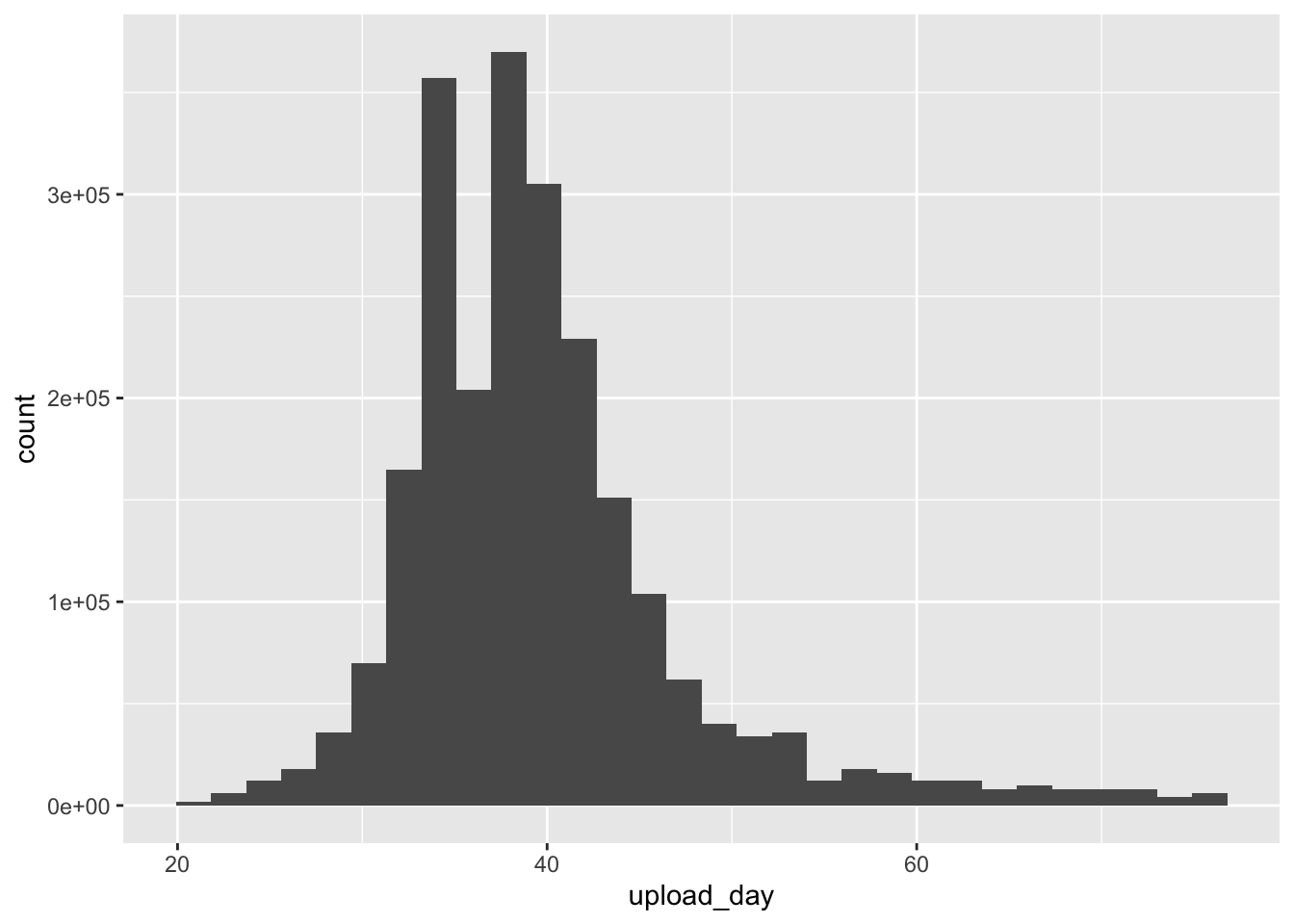
ggplot2::ggplot(ice_tib, aes(upload_day))+geom_histogram(binwidth =1, fill ="#440154", alpha =0.25)+labs(y ="Frequency", x ="Days since first ice bucket challenge video")
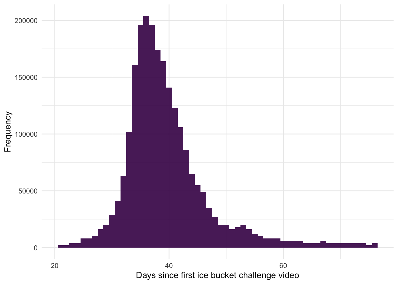
Themes
Show the code
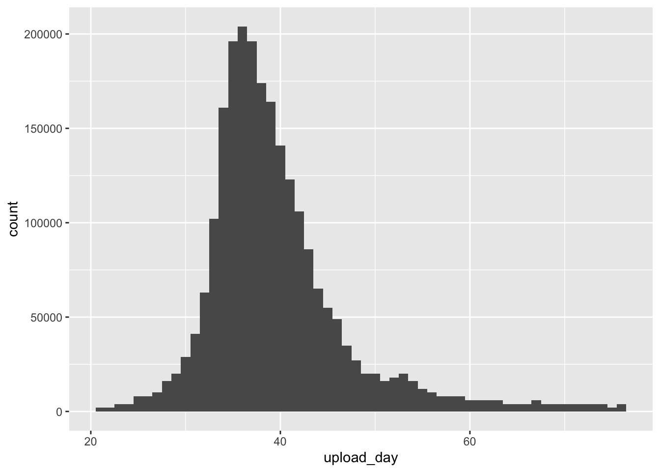
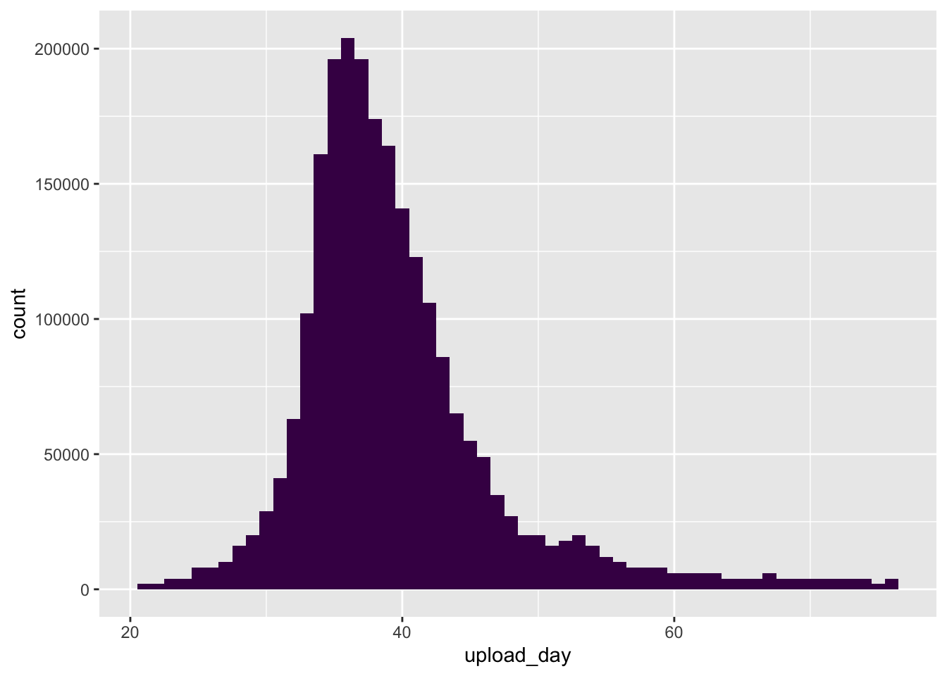
ggplot2::ggplot(ice_tib, aes(upload_day))+geom_histogram(binwidth =1, fill ="#440154", alpha =0.9)+labs(y ="Frequency", x ="Days since first ice bucket challenge video")+theme_minimal()
Summarizing data
Mean and median
mean(variable, trim = 0, na.rm = FALSE)
trim
allows you to trim scores before calculating the mean by specifying a value between 0 and 0.5. default is 0 (no trim). to trim 10% of scores fom each end of the distribution you could set trim = 0.1
na.rm
stands for NA remove. Missing values are denoted NA, for ‘not available’. by setting na.rm = TRUE (or na.rm = T), R will remove missing values before computing the mean
TipMissing Values
The default in many functions is not to remove missing values (e.g. na.rm = FALSE). If you have missing values in your data and don’t change this default behaviour R will throw an error. Therefore, if you get an error from a function like mean(), check whether you have missing values and whether you have forgotten to set na.rm = TRUE.
The function for median is similar, except no trim (median is effectively the mean with 50% trim)
median(variable, na.rm = FALSE)
Code example
if the defaults are ok, there is no need to set those arguments
Use what you learned in the previous section and the code example above to get the variance and standard deviation of the days since the original ice bucket video that other videos were uploaded.
ice_tib |>
  dplyr::summarise(
    median =  median(upload_day),  # creates new variable called `median` from the output of `median(upload_day)`
    mean =  mean(upload_day), # creates new variable called `mean` from the output of `mean(upload_day)`
    ...
    )
coding challenge
Create a summary table containing the mean, median, IQR, variance and SD of the number of days since the original ice bucket video.
Show the code
ice_tib|>dplyr::summarise( median =median(upload_day), # creates new variable called `median` from the output of `median(upload_day)` mean =mean(upload_day), # creates new variable called `mean` from the output of `mean(upload_day)` IQR =IQR(upload_day), var =var(upload_day), sd =sd(upload_day))
# A tibble: 1 × 5
  median  mean   IQR   var    sd
   <dbl> <dbl> <dbl> <dbl> <dbl>
1     38  39.7     7  59.9  7.74
Code example
To store the summary of stats, we assign it to a new object:
Show the code
upload_summary<-ice_tib|>dplyr::summarise( median =median(upload_day), mean =mean(upload_day), IQR =IQR(upload_day), variance =var(upload_day), std_dev =sd(upload_day))upload_summary
# A tibble: 1 × 5
  median  mean   IQR variance std_dev
   <dbl> <dbl> <dbl>    <dbl>   <dbl>
1     38  39.7     7     59.9    7.74
Rounding Values
use round() function to round values and use kable() from knitr to round an entire table of values