Rows: 500 Columns: 4
── Column specification ────────────────────────────────────────────────────────
Delimiter: ","
chr (2): strategy, time
dbl (2): id, success

ℹ Use `spec()` to retrieve the full column specification for this data.
ℹ Specify the column types or set `show_col_types = FALSE` to quiet this message.
Rows: 40 Columns: 3
── Column specification ────────────────────────────────────────────────────────
Delimiter: ","
chr (2): sex, film
dbl (1): arousal

ℹ Use `spec()` to retrieve the full column specification for this data.
ℹ Specify the column types or set `show_col_types = FALSE` to quiet this message.
Rows: 103 Columns: 5
── Column specification ────────────────────────────────────────────────────────
Delimiter: ","
chr (1): sex
dbl (4): id, revise, exam_grade, anxiety

ℹ Use `spec()` to retrieve the full column specification for this data.
ℹ Specify the column types or set `show_col_types = FALSE` to quiet this message.
need to turn categorical variables into factors
Show the code
wish_tib<-wish_tib|>dplyr::mutate( strategy =forcats::as_factor(strategy), time =forcats::as_factor(time)|>forcats::fct_relevel("Baseline"))
Show the code
notebook_tib<-notebook_tib|>dplyr::mutate( sex =forcats::as_factor(sex), film =forcats::as_factor(film))
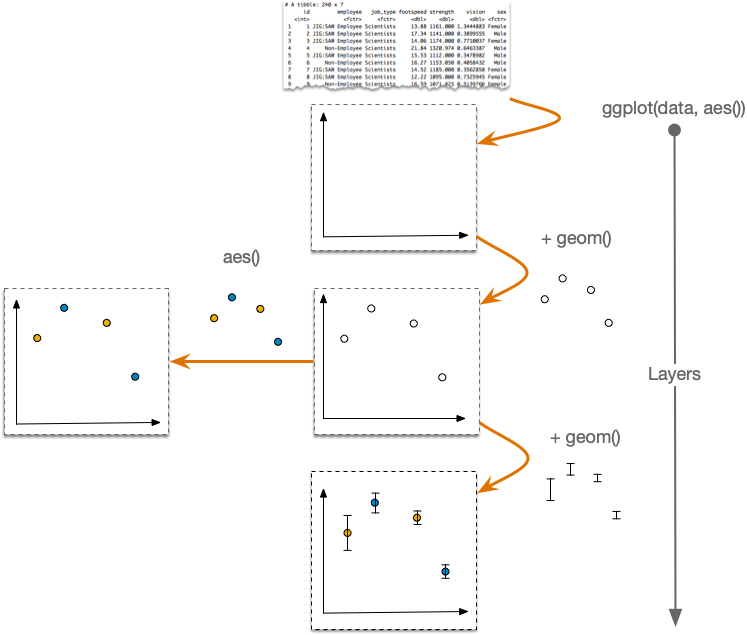
some situations where it is easier to display a summary of the data directly to the plot (usually stat_summary())
Scales
control details of how data are mapped to their visual objects to control what appears on x and y axes using scale_x_continuous() and scale_y_continuous(), axis labels are controlled with labs()
Each of the above are layers that can be added to a plot, as below
Explanation of the layered approach to ggplot2
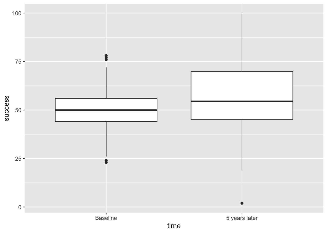
Boxplots (box-whisker plots)
imaginary data based on peoples’ level of success (0-100)
one group told to wish for good success, other group told to work hard for success
measured success again 5 years later
The data are in wish_tib. The variables are id (the person’s id), strategy (hard work or wishing upon a star), time (baseline or 5 years), and success (the rating on my dodgy scale).
wish_plot<-ggplot2::ggplot(wish_tib, aes(time, success))# creates an object called `wish_plot` that contains the boxplot# ggplot() function specifies the plot will use `wish_tib` and plots time on *x* and success on *y*wish_plot+geom_boxplot()# adds boxplot geom to wish_plot
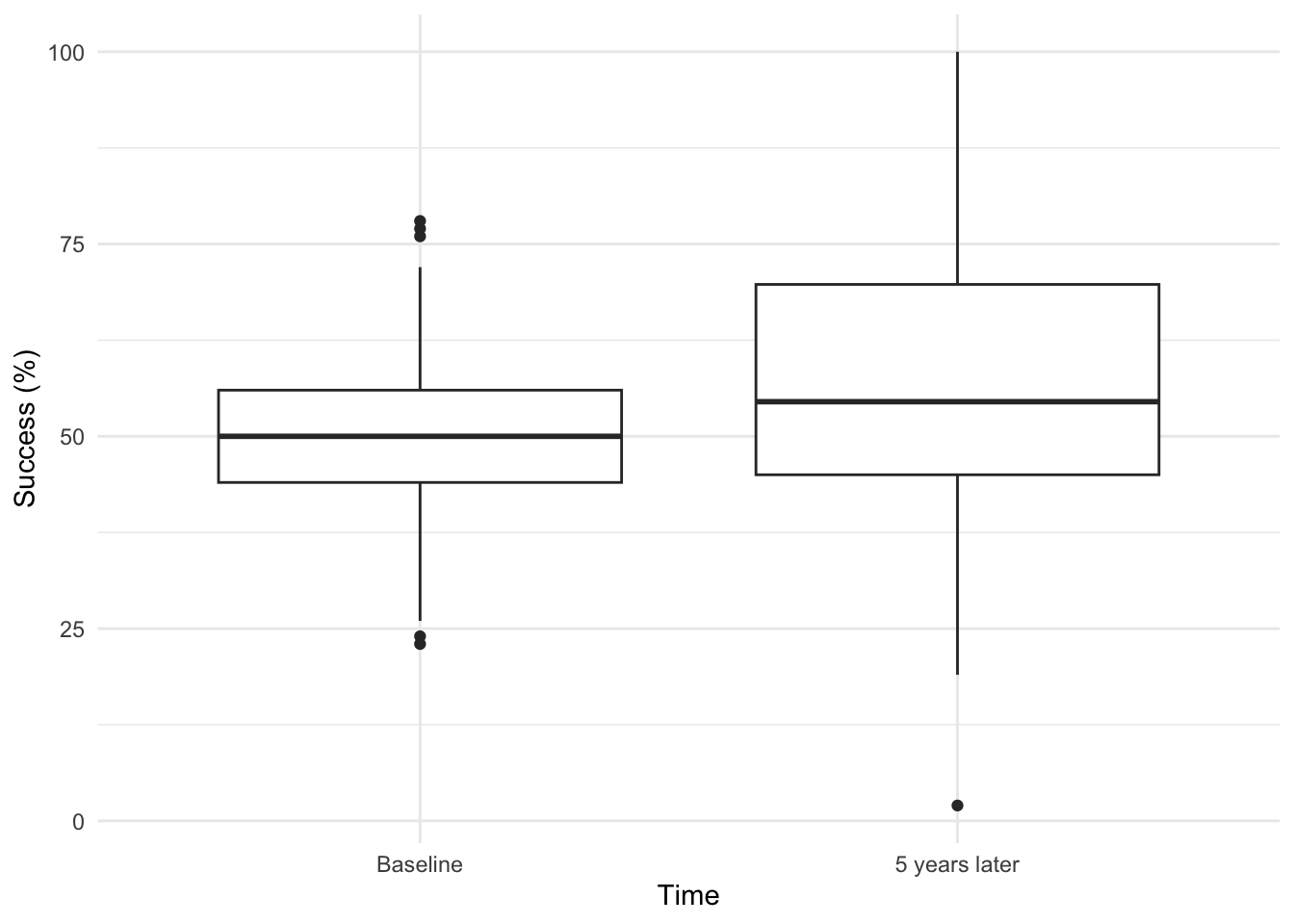
Show the code
wish_plot<-ggplot2::ggplot(wish_tib, aes(time, success))wish_plot+geom_boxplot()+labs(x ="Time", y ="Success (%)")+# add labels to axestheme_minimal()# add minimal theme layer
plot shows slight increase of success, but doesn’t show the effect of hard work