Rows: 68 Columns: 4
── Column specification ────────────────────────────────────────────────────────
Delimiter: ","
chr (2): id, novice
dbl (2): creativity, position

ℹ Use `spec()` to retrieve the full column specification for this data.
ℹ Specify the column types or set `show_col_types = FALSE` to quiet this message.
Rows: 103 Columns: 5
── Column specification ────────────────────────────────────────────────────────
Delimiter: ","
chr (1): sex
dbl (4): id, revise, exam_grade, anxiety

ℹ Use `spec()` to retrieve the full column specification for this data.
ℹ Specify the column types or set `show_col_types = FALSE` to quiet this message.
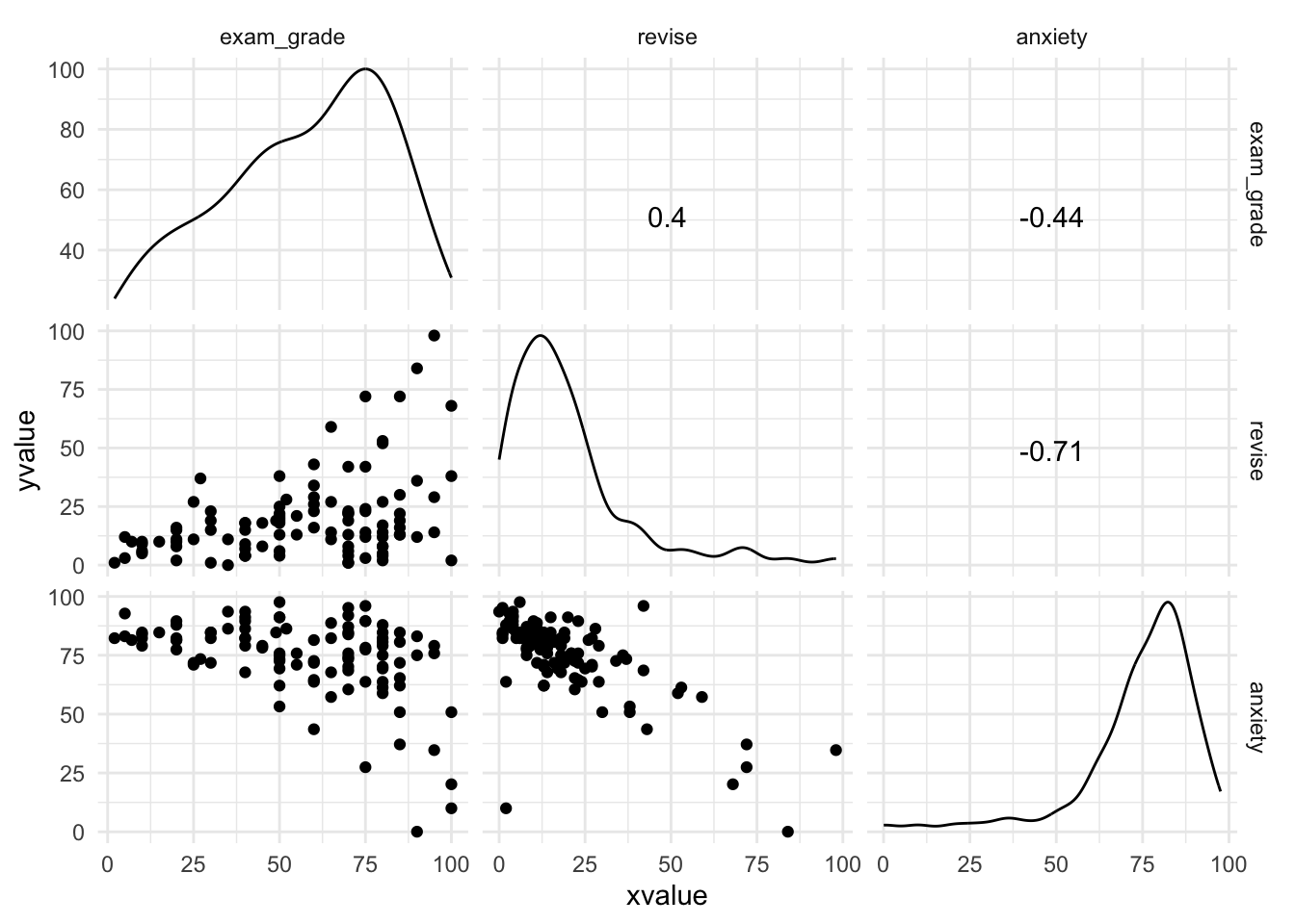
plot continuous variables, the ggscatmat() function produces a matrix of scatterplots (below the diagonal), distributions (along the diagonal) and the correlation coefficient (above the diagonal)
should be replaced with the name of tibble containing any variables to correlate
method
method of correlation coefficient, default is pearson, but can also accept spearman, kendall, biserial, polychoric, tetrachoric, and percentage
p_adjust
corrects the \(p\)-value for the number of tests you have performed using the Holm-Bonferroni method
applies the Bonferroni criterion in a slightly less strict way that controls the type I error, but with less risk of a type II error
can change to none (bad idea), bonferroni (to apply the standard Bonferroni method) or several other methods.
ci
set the confidence interval width; default is 0.95 for general use
To use the function, - pipe tibble into the select() function from dplyr to select variables to correlate, then pipe that into the correlation function - use the same syntax whether you want to correlate two variables or produce all correlations between pairs of multiple variables]
To calculate Pearson correlation btwn variables exam_grade and revise in exam_tib…
ImportantThe confidence interval for the association between exam grade and revision is 0.22 to 0.55. What does this tell us?
If this confidence interval is one of the 95% that contains the population value then the population value of r lies between 0.22 and 0.55.
ImportantThe p-value for the association between exam grade and revision is < 0.001, what does this value mean?
The probability of getting a value of t at least as big as the value we have observed, if the value of r were, in fact, zero is less than 0.001. I’m going to assume, therefore, that the association between exam grade and revision is not zero.
exam grade correlates with revision - \(r\)=0.4
exam grade had a similar strength relationship with exam anxiety \(r\)=-0.44 but in the opposite direction
revision had a strong negative relationship with anxiety - \(r\)=-0.709
the more you revise, the better your performance
the more anxiety you have, the worse your performance
the mopre you revise, the less anxiety you have
all \(p\)-values are less than 0.001 and would be interpreted as the correlation coefficients being significantly different from zero
significance values tell us that the probability of getting correlation coefficients at least as big as this in a sample of 103 people if the null were true (that there was no relationship between the variables) is very low
if we assume the sample is one of the 95% of samples that will produce a confidence interval containing the population value, then the confidence intervals tell us about the uncertainty around \(r\).
TipRounding
We can control the number of decimal places using knitr::kable(digits = 3)
We can also specify different columns to contain different rounding using knitr::kable(digits = c(2, 2, 2, 2, 2, 2, 2, 2, 8)) (column 9 to 8 decimal places) or knitr::kable(digits = c(rep(2, 8), 8))
Robust correlation coefficients
Given the skew in the variables, we should use a robust correlation coefficient, like the percentage bend correlation coefficient by setting method = "percentage" within correlation()
All robust correlations (percentage bend) are less than raw, though all are significant at \(p<0.001\)
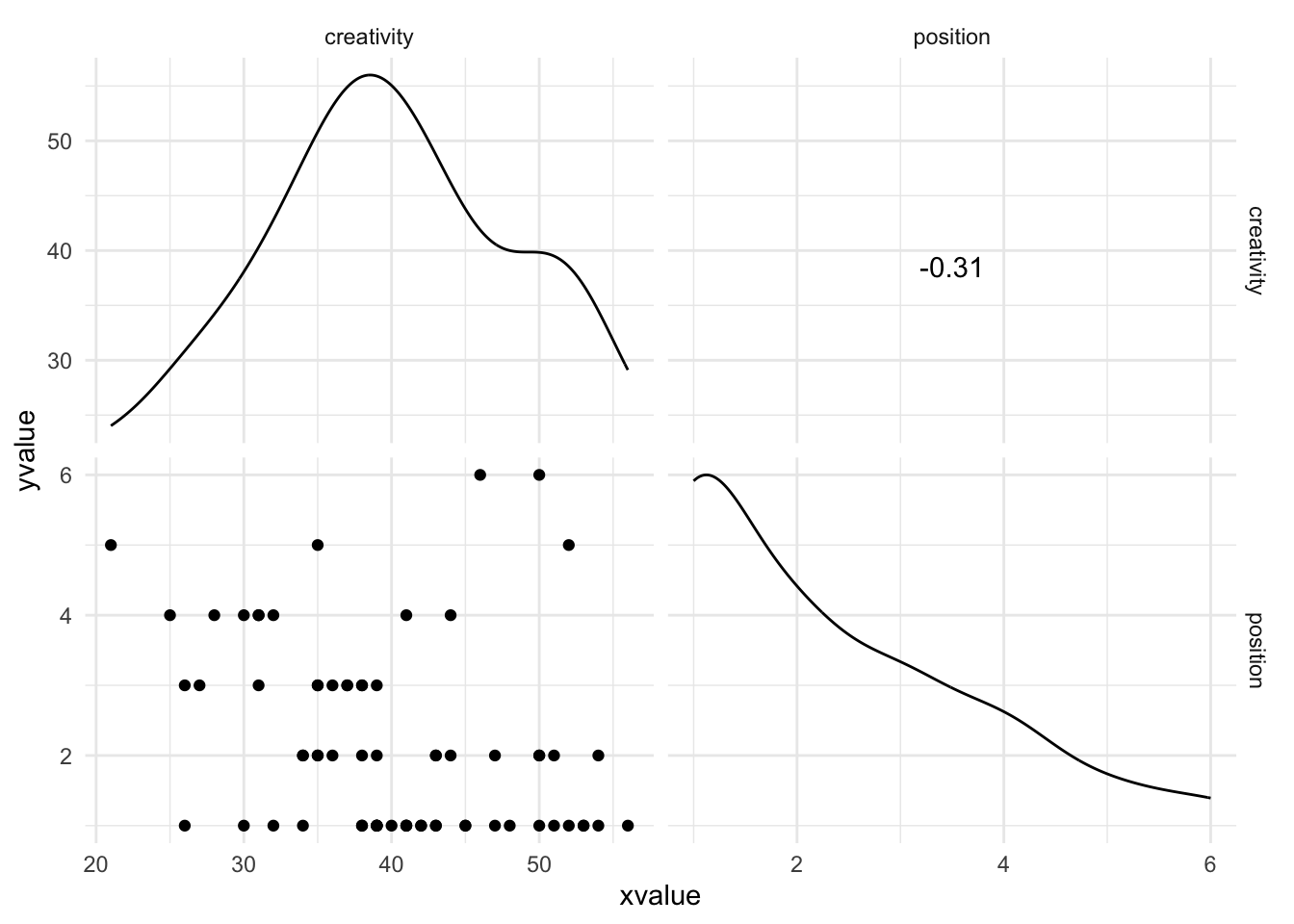
Spearman’s correlation coefficient
data from World’s Best Liar competition
want to know if creativity impacts lying ability
position data (1st, 2nd, etc) is ordinal, so Spearman’s correlation coefficient should be used
Data are in
Show the code
liar_tib
# A tibble: 68 × 4
   id    creativity position novice
   <chr>      <dbl>    <dbl> <fct>
 1 lnwe          53        1 First time
 2 vxob          36        3 Previous entrant
 3 qpli          31        4 First time
 4 pwsq          43        2 First time
 5 xafq          30        4 Previous entrant
 6 njra          41        1 First time
 7 lxty          32        4 First time
 8 dxcw          54        1 Previous entrant
 9 uxgp          47        2 Previous entrant
10 dvew          50        2 First time
# ℹ 58 more rows
output shows \(\tau=-0.3\) -> closer to 0 than Spearman (-.38) therefore Kendall’s value is likely a more accurate guage of what the correlation in the population would be