discovr_08 - General Linear Model

library(tidyverse, ggplot2)

── Attaching core tidyverse packages ──────────────────────── tidyverse 2.0.0 ──
✔ dplyr     1.1.4     ✔ readr     2.1.5
✔ forcats   1.0.0     ✔ stringr   1.5.1
✔ ggplot2   3.5.1     ✔ tibble    3.2.1
✔ lubridate 1.9.3     ✔ tidyr     1.3.1
✔ purrr     1.0.2     
── Conflicts ────────────────────────────────────────── tidyverse_conflicts() ──
✖ dplyr::filter() masks stats::filter()
✖ dplyr::lag()    masks stats::lag()
ℹ Use the conflicted package (<http://conflicted.r-lib.org/>) to force all conflicts to become errors

library(ggfortify)
library(robust)

Loading required package: fit.models

album_tib <- here::here("data/album_sales.csv") |> readr::read_csv()

Rows: 200 Columns: 5
── Column specification ────────────────────────────────────────────────────────
Delimiter: ","
chr (1): album_id
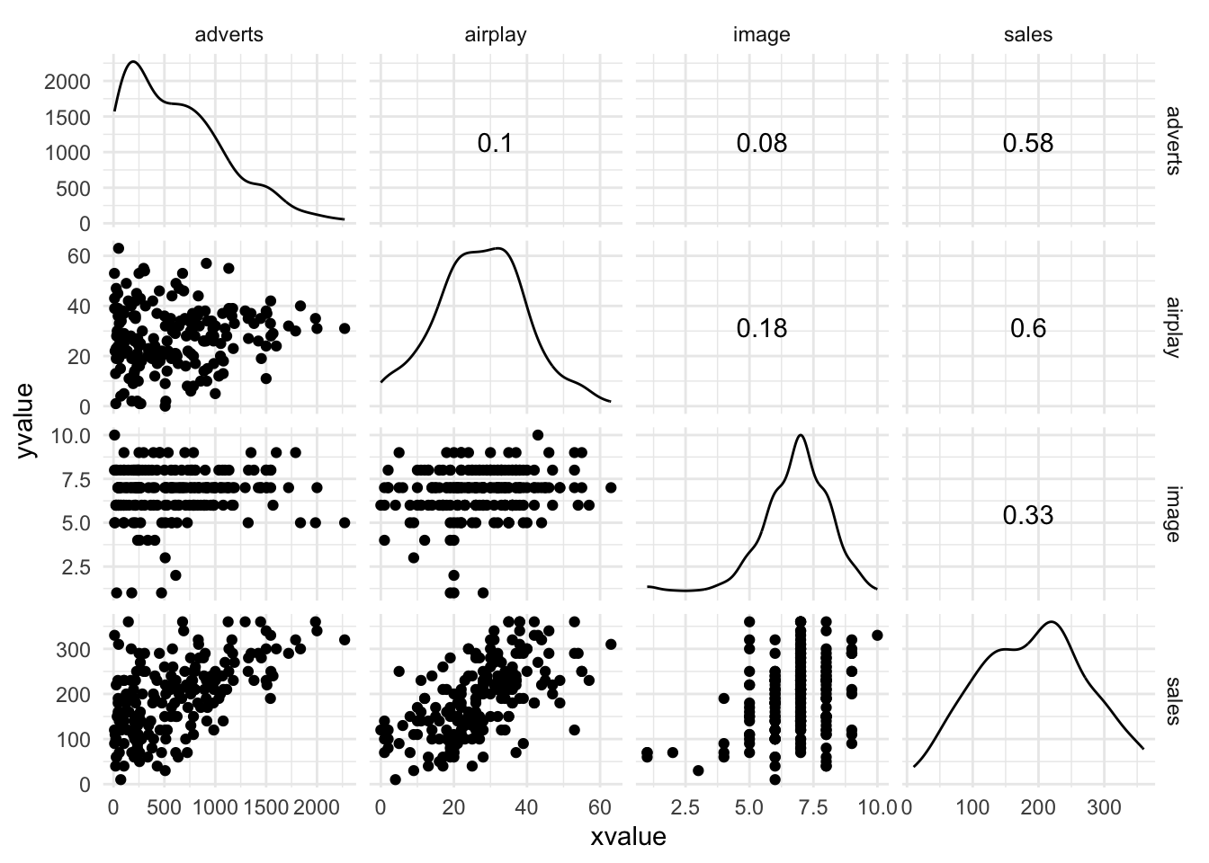
dbl (4): adverts, sales, airplay, image

ℹ Use `spec()` to retrieve the full column specification for this data.
ℹ Specify the column types or set `show_col_types = FALSE` to quiet this message.

soc_anx_tib <- here::here("data/social_anxiety.csv") |> readr::read_csv()

Rows: 134 Columns: 4
── Column specification ────────────────────────────────────────────────────────
Delimiter: ","
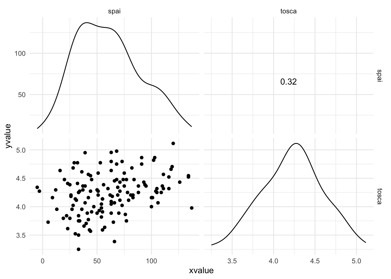
dbl (4): spai, iii, obq, tosca

ℹ Use `spec()` to retrieve the full column specification for this data.
ℹ Specify the column types or set `show_col_types = FALSE` to quiet this message.

metal_tib <- here::here("data/metal_health.csv")  |> readr::read_csv()

Rows: 2506 Columns: 2
── Column specification ────────────────────────────────────────────────────────
Delimiter: ","
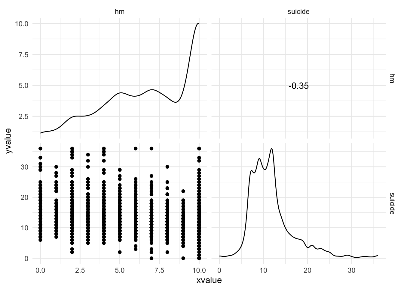
dbl (2): hm, suicide

ℹ Use `spec()` to retrieve the full column specification for this data.
ℹ Specify the column types or set `show_col_types = FALSE` to quiet this message.

Fitting the Linear Model

• scatterplots to get an idea of whether assumption of linearity is met, look for outliers or other unusual cases
• run an initial regression and save the diagnostics
• if we want to generalize or test for significance or confidence intervals…
  • examine residuals for homoscedasticity, independence, normality, and linearity
    • lack of linearity –> fit a non-linear model
    • assumptions met and no bias –> Model can be generalized
    • lack of independent errors –> multi-level model
    • all other situations –> fit a robust version of the model using bootstrapping (small samples) or robust standard errors

homoscedasticity

assumption of equal or similar variances in different groups being compared

homogeneity of variance

Figure 1

album_tib

# A tibble: 200 × 5
   album_id adverts sales airplay image
   <chr>      <dbl> <dbl>   <dbl> <dbl>
 1 aox1foms    10.3   330      43    10
 2 u453js2i   986.    120      28     7
 3 pie89xnr  1446.    360      35     7
 4 u2k5a0df  1188.    270      33     7
 5 t4699ux3   575.    220      44     5
 6 s4h49cu2   569.    170      19     5
 7 1235a8sf   472.     70      20     1
 8 p2v24p5k   537.    210      22     9
 9 4fbjg024   514.    200      21     7
10 e9w6usdb   174.    300      40     7
# ℹ 190 more rows

• Use GGally::ggscatmat package to visualize the data
• produces
  • a matrix of scatterplots below the diagonal
  • distributions along the diagonal
  • the correlation coefficient above the diagonal

GGally::ggscatmat(album_tib, columns = c("adverts", "airplay", "image", "sales"))  +
theme_minimal()

Registered S3 method overwritten by 'GGally':
  method from   
  +.gg   ggplot2

Interpretation

• 3 predictors have reasonably linear relationships with album sales and no obvious outliers (except bottom left of ‘band image’ scatterplots)
• across the diagonal (distributions)
  • advertising is very skewed
  • airplay and sales look heavy-tailed
• correlations in the plot give us an idea of the relationships between predictors and outcome
• if we ignore album sales, the highest correlation is between image ratings and amount of airplay, which is significant and the 0.01 level (\(r=0.18\))
• focussing on the outcome variable, adverts and airplay correlate best with the outcome (\(r=0.58\) and \(r=0.6\))

One predictor

Fitting the model

• predicting sales from advertising alone

\[Y_i=b_0+{b_1}{X_i}+\epsilon_i\]

\[\text{Sales}_i=b_0+{b_1}{\text{Advertising}_i}+\epsilon_i\]

• it is clear from the bottom left scatterplot and the correlation (\(r=0.58\)) that a positive relation exists. More advertising money spent leads to greater album sales.
• some albums sell well regardless of advertising (top-left of scatterplot)
• no albums sell badly when adverts are high (bottom-right of scatterplot)
• to fit a linear model, we use lm() function my_model <- lm(outcome ~ predictor(s), data = tibble, na.action = an action)
  • my_model is the name of the model
  • outcome is the name of the outcome variable (sales)
  • predictor is the name of the predictor variable (adverts) or, a list of variables separated by + symbols
  • tibble is the name of the tibble containing the data (album_tib)
• this function maps directly to the equation for the model
  • adverts ~ sales maps to \(\text{Sales}_i=b_0+{b_1}{\text{Advertising}_i}+\epsilon_i\) except we ignore the error term and parameter estimates and we replace the = with ~ (which means ‘predicted from’)

album_lm <- lm(sales ~ adverts, data = album_tib, na.action = na.exclude)
summary(album_lm)

Call:
lm(formula = sales ~ adverts, data = album_tib, na.action = na.exclude)

Residuals:
     Min       1Q   Median       3Q      Max 
-152.949  -43.796   -0.393   37.040  211.866 

Coefficients:
             Estimate Std. Error t value Pr(>|t|)    
(Intercept) 1.341e+02  7.537e+00  17.799   <2e-16 ***
adverts     9.612e-02  9.632e-03   9.979   <2e-16 ***
---
Signif. codes:  0 '***' 0.001 '**' 0.01 '*' 0.05 '.' 0.1 ' ' 1

Residual standard error: 65.99 on 198 degrees of freedom
Multiple R-squared:  0.3346,    Adjusted R-squared:  0.3313 
F-statistic: 99.59 on 1 and 198 DF,  p-value: < 2.2e-16

broom::glance(album_lm)  |> 
  knitr::kable(digits = 3)

r.squared	adj.r.squared	sigma	statistic	p.value	df	logLik	AIC	BIC	deviance	df.residual	nobs
0.335	0.331	65.991	99.587	0	1	-1120.688	2247.375	2257.27	862264.2	198	200

• note \(df=1\) and \(df.residual=198\) therefore we can say that adding the predictor of advertising significantly improved the fit of the model to the data compared to having no predictors in the model
• \(F(1,198)=99.59, p<.001\)

Model Parameters

To see model parameters, use broom::tidy()

broom::tidy(model_name, conf.int = FALSE, conf.level = 0.95)

• put the model name into the function, then two optional arguments
  • confidence intervals conf.int=TRUE (confidence intervals are not included by default)
  • default is 95%, but you can change it with conf.level=.99 for 99% confidence interval

broom::tidy(album_lm, conf.int = TRUE)

# A tibble: 2 × 7
  term        estimate std.error statistic  p.value conf.low conf.high
  <chr>          <dbl>     <dbl>     <dbl>    <dbl>    <dbl>     <dbl>
1 (Intercept) 134.       7.54        17.8  5.97e-43 119.       149.   
2 adverts       0.0961   0.00963      9.98 2.94e-19   0.0771     0.115

• output provides estimates of the model parameters (\(\hat{b}\)-values)
• \(Y\) intercept (\(b_0\)) is 134.14 (when \(X\) is 0, sales will be 134140)
• \(X\) (\(b_1\)) is 0.096.
  • represents the change in outcome associated with a unit change in predictor.
  • when the predictor increases by 1, the outcome increases by .096, but since the units of measurement was thousands of pounds and thousands of sales, an increase in $1000 will lead to 96 more albums sold
  • not very good return
  • BUT, we know that advertising only accounts for 1/3 of the variance
• If a predictor is having a significant impact on our ability to predict the outcome, then \(\hat{b}\) should be different from 0 and large relative to its standard error
• the \(t\)-test (labelled statistic) and the associated \(p\)-value tell us whether the \(\hat{b}\) is significantly different from 0
• the column p.value contains the exact probability that a value of \(t\) at least as big as the one in the table would occur if the value of \(b\) in the population were 0
• if this propbability is less than 0.05, then we interpret that as the predictor being a significant predictor of hte outcome.
• for both \(t\)s, the probabilities are in scientific notation
  • 2.91e-19 means \(2.91*10^{-19}\), or move the decimal 19 places to the left or 0.000000000000000000291
  • 2.91e+19 means \(2.91*10^{19}\), or move the decimal 19 places to the right or 29100000000000000000
    
• both values are 0 at 3 decimal places

Exploring the standard error of \(\hat{b}\)

https://www.youtube-nocookie.com/embed/3L9ZMdzJyyI?si=ET90VDYq3RVKnKDq

Confidence intervals for \(\hat{b}\)

Imagine we collect 100 samples of data measuring the same variables as the current model, then estimate the same model, including confidence intervals for unstandardized values.The boundaries are constructed such that 95% of our 100 samples contain the population value of \(b\). 95 of 100 sample will yield confidence intervals for \(b\) that contain the population value, but we don’t know if our sample is one of the 95.

We might just assume that it does, but if the confidence interval contains 0, then there is a possibility that there is no relationship, or the relationship might be negative. The trouble is that we would be wrong 5% of the time.

If the interval does not contain 0, we might conclude there is a genuine positive relationship.

Using the model

\[\text{Sales}_i=\hat{b_0}+\hat{b_1}{\text{Advertising}_i}\]

\[\text{Sales}_i=134.14+.096*{Advertising}_i\]

Now we can make a prediction by entering a value for the advertising budget, say 100 (equal to 100,000 gbp)

\[\text{Sales}_i=134.14+.096*{100}_i\]

\[\text{Sales}_i=143.74\]

or 143,740 sales

Several Predictors

add multiple predictors hierarchically, after advertising is shown to be significant

\[Y_i=b_0+{b_1}{X_1i}+{b_2}{X_2i}+{b_3}{X_3i}+ ... +{b_n}{X_ni}\epsilon_i\]

\[Y_i=b_0+{b_1}{advertising_i}+{b_2}{airplay_i}+{b_3}{image_i}+\epsilon_i\]

Building the model

• add predictors to the R code the same way as we do in the equation, by adding +

album_full_lm <- lm(sales ~ adverts + airplay + image, data = album_tib, na.action = na.exclude)
summary(album_full_lm)

Call:
lm(formula = sales ~ adverts + airplay + image, data = album_tib, 
    na.action = na.exclude)

Residuals:
     Min       1Q   Median       3Q      Max 
-121.324  -28.336   -0.451   28.967  144.132 

Coefficients:
              Estimate Std. Error t value Pr(>|t|)    
(Intercept) -26.612958  17.350001  -1.534    0.127    
adverts       0.084885   0.006923  12.261  < 2e-16 ***
airplay       3.367425   0.277771  12.123  < 2e-16 ***
image        11.086335   2.437849   4.548 9.49e-06 ***
---
Signif. codes:  0 '***' 0.001 '**' 0.01 '*' 0.05 '.' 0.1 ' ' 1

Residual standard error: 47.09 on 196 degrees of freedom
Multiple R-squared:  0.6647,    Adjusted R-squared:  0.6595 
F-statistic: 129.5 on 3 and 196 DF,  p-value: < 2.2e-16

broom::glance(album_full_lm)  |> 
  knitr::kable(digits = 3)

r.squared	adj.r.squared	sigma	statistic	p.value	df	logLik	AIC	BIC	deviance	df.residual	nobs
0.665	0.66	47.087	129.498	0	3	-1052.168	2114.337	2130.828	434574.6	196	200

• r.squared \(R^2\) tells us the variance in album sales -> .665, or 66.5%.
• \(R^2\) for adverts was 0.335, so the difference -> .665-.335=.33 means that airplay and image account for a further 33% of the variance
• adjusted \(R^2\) adj.r.squared tells us how well the model generalizes, and the value should be close to r.squared.
  • in this case it is .66, or only .005 away
• \(F\)-statistic is the ratio of the improvementin prediction that results from fitting the model, relative to the inaccuracy that sitll exists in the model
• the variable p.value contains the p-value associated with \(F\) -> in this case is \(2.88×10^{−46}\) -> much smaller than .001
• degrees of freedom are df and df.residual
• we can interpret the result as meaning that the model significantly improves our ability to predict the outcome variable ocmpared to not fitting the model.
• reported as \(F(3, 196)=129.5, p=<0.001\)

Comparing Models

• we can compare hierarchical models using an \(F\)-statisticusing the anova() function -> anova(model_1, model_2, … , model_n)
• list the models in order that we want to compare

anova(album_lm, album_full_lm) |>
broom::tidy()

# A tibble: 2 × 7
  term                      df.residual    rss    df   sumsq statistic   p.value
  <chr>                           <dbl>  <dbl> <dbl>   <dbl>     <dbl>     <dbl>
1 sales ~ adverts                   198 8.62e5    NA     NA       NA   NA       
2 sales ~ adverts + airpla…         196 4.35e5     2 427690.      96.4  6.88e-30

• \(F\) (statistic) is 96.5
• \(p\)-value (p.value) is \(6.8793949^{-30}\)
• df is 2 (difference between df in 2 models)
• df.residual is 196
• Conclusion -> adding airplay and image to the model significantly improved model fit
  • \(F(2, 196) = 96.45, p < 0.001\)

Tip

We can only compare hierarchical models; that is to say that the second model must contain everything that was in the first model plus something new, and the third model must contain everything in the second model plus something new, and so on.

Model parameter estimates (\(\hat{b}\))

broom::tidy(album_full_lm, conf.int = TRUE)  |> 
  knitr::kable(digits = 3)

term	estimate	std.error	statistic	p.value	conf.low	conf.high
(Intercept)	-26.613	17.350	-1.534	0.127	-60.830	7.604
adverts	0.085	0.007	12.261	0.000	0.071	0.099
airplay	3.367	0.278	12.123	0.000	2.820	3.915
image	11.086	2.438	4.548	0.000	6.279	15.894

• output gives estimates of the \(b\)-balues (column labelled estimate) and statistics that indicate the individual contribution of each predictor in the model.
• all three predictors have positive \(\hat{b}\)values, indicating positive relationships
  • as all three predictors increase, so do album sales
• \(\hat{b}\) vlaues also tell us to what degree each predictor affects the outcome if the effects of all other predictors are held constant
  • advertising budget -> \(\hat{b}=0.085\) -> as advertising increases by 1 unit (1000gbp), sales increases by 0.085 units (85 albums), but this is only true if the other two predictors are held constant
  • airplay \(\hat{b}=3.367\) -> as airplay prior to release increases by one unit (1 play), album sales increase by 3.367 units (3367 album sales, but only if the other two predictors are held constant)

How would we interpret the 𝑏̂ (11.086) for band image?

If a band can increase their image rating by 1 unit they can expect additional album sales of 11,086 units

Standardized \(\hat{b}\)s

The lm() function does not provide standardized betas, so use model_parameters()

parameters::model_parameters(my_model, standardize = refit)

parameters::model_parameters(album_full_lm, standardize = "refit") |> 
  knitr::kable(digits = 3)

Parameter	Coefficient	SE	CI	CI_low	CI_high	t	df_error	p
(Intercept)	0.000	0.041	0.95	-0.081	0.081	0.000	196	1
adverts	0.511	0.042	0.95	0.429	0.593	12.261	196	0
airplay	0.512	0.042	0.95	0.429	0.595	12.123	196	0
image	0.192	0.042	0.95	0.109	0.275	4.548	196	0

• advertising budget -> Standardized \(\hat{\beta}=0.511\)
  • as the advertising budgetr increases by one standard deviation (485,655gbp), album sales increase by .511 standard deviations.
  • the standard deviation for album sales is 80,699, so .511 SD is 41,240 sales
  • for every increase in advert budget of 485655gbp, album sales will increase by 41,240 IF the other predictors are held constant
• Image -> Standardized \(\hat{\beta}=0.192\)
  • a band rated 1 SD on the image scale (1.4 units) will sell .192 SD more units.
  • this is a change of 15,490 sales IF the other predictors are held constant

How would we interpret the Standardized B (0.512) for airplay?

As the number of plays on radio in the week before release increases by 1 standard deviation, album sales increase by 0.512 standard deviations

Confidence Intervals

The confidence interval for airplay ranges from 2.82 to 3.92. What does this tell us?

• The probability of this confidence interval containing the population value is 0.95.
• If this confidence interval is one of the 95% that contains the population value then the population value of b lies between 2.82 and 3.92.
• I can be 95% confident that the population value of b lies between 2.82 and 3.92
• There is a 95% chance that the population value of b lies between 2.82 and 3.92

Assuming that each confidence interval is one of the 95% that contains the population parameter: - the true size of the relationship between advertising budget and album sales lies somewhere between 0.071 and 0.099 - the true size of the relationship between band image and album sales lies somewhere between 6.279 and 15.894

• the two best predictors have tight confidence intervals (airplay and adverts) indicating that the estimates are likely representative of the true population values
• the interval for band image is much wider, but does not cross zero indicating this parameter is less representative of the population, but is still significant.

Significance tests

The values in statistic are the values of \(t\) associated with each \(\hat{b}\) and p.value is the associated significance of the \(t\)-statistic. For every predictor, the \(\hat{b}\) is significantly different from 0 (\(p<.001\)) meaning that all predictors significantly predict album sales.

How might we interpret the statistic and p.value for the three predictors?

• The probability of the null hypothesis is less than 0.001 in all cases
• The probability that each b is a chance result is less than 0.001
• They tell us that the probability of getting a value of t at least as big as these values if the value of b were, in fact, zero is smaller than 0.001 for all predictors.

\(p\)-values

Many students and researchers think of p-values in terms of the ‘probability of a chance result’ or ‘the probability of a hypothesis being true’ but they are neither of these things. They are the long-run probability that you would get a test-statistic (in this case t) at least as large as the one you have if the null hypothesis were true. In other words, if there really were no relationship between advertising budget and album sales (the null hypothesis) then the population value of b would be zero.

Imagine we sampled from this null population and computed t, and then repeated this process 1000 times. We’d have 1000 values of t from a population in which there was no effect. We could plot these values as a histogram. This would tell us how often certain values of t occur. From it we could work out the probability of getting a particular value of t. If we then took another sample, and computed t (because we’re kind of obsessed with this sort of thing) we would be able to compare this value of t to the distribution of all the previous 1000 samples. Is the t in our current sample large of small compared to the others? Let’s say it was larger than 999 of the previous values. That would be quite an unlikely value of t whereas if it was larger than 500 of them this would not surprise us. This is what a p-value is: it is the long run probability of getting test statistic at least as large as the one you have if the null hypothesis were true. If the value is less than 0.05, people typically take this as supporting the idea that the null hypothesis isn’t true.

Report

• the model that included the band’s image and airplay was significantly better fit than the model that included advertising budget alone \(f(2, 196)=96.45, p<0.001\)
• the final model explained 66.5% of the variance in album sales
• advertising budget significantly predicted album sales \(\hat{b}=0.08[0.07, 0.10], t(196)=12.26, p>.001\)
• airplay significantly predicted album sales \(\hat{b}=3.37[2.82, 3.92], t(196)=12.12, p<.001\)
• band image significantly predicted album sales -> \(\hat{b}=11.09[6.28, 15.89], t=4.55, p<.001\)

Unguided Example

Metal and mental health

metal_tib

# A tibble: 2,506 × 2
      hm suicide
   <dbl>   <dbl>
 1    10       7
 2    10      11
 3    10       8
 4     4      14
 5    10      13
 6     8      12
 7     8       7
 8     5      15
 9     8       7
10     9      10
# ℹ 2,496 more rows

GGally::ggscatmat(metal_tib, columns=c("hm", "suicide")) + theme_minimal()

Warning: Removed 200 rows containing non-finite outside the scale range
(`stat_density()`).

Warning: Removed 284 rows containing non-finite outside the scale range
(`stat_density()`).

metal_lm <- lm(suicide ~ hm, data = metal_tib, na.action = na.exclude)
broom::glance(metal_lm) |>
knitr::kable(digits=3)

r.squared	adj.r.squared	sigma	statistic	p.value	df	logLik	AIC	BIC	deviance	df.residual	nobs
0.125	0.125	4.842	304.784	0	1	-6401.851	12809.7	12826.7	50047.05	2135	2137

broom::tidy(metal_lm, conf.int = TRUE, conf.level=0.95)

# A tibble: 2 × 7
  term        estimate std.error statistic  p.value conf.low conf.high
  <chr>          <dbl>     <dbl>     <dbl>    <dbl>    <dbl>     <dbl>
1 (Intercept)   16.0      0.261       61.4 0          15.5      16.5  
2 hm            -0.612    0.0350     -17.5 6.64e-64   -0.680    -0.543

How much variance does the final model explain?

12.5%

What is the nature of the relationship between listening to heavy metal and suicide risk?

• As love of heavy metal increases, suicide risk decreases
• because the \(\hat{b}\) value is negative (-.0612)

As listening to heavy metal increases by 1 unit, by how much does suicide risk change?

• -0.612 units

Predicting Social Anxiety

soc_anx_tib

# A tibble: 134 × 4
    spai   iii   obq tosca
   <dbl> <dbl> <dbl> <dbl>
 1    26 56.5   4.43  4.18
 2    51 16.1   2.03  4.20
 3    33 37.4   2.59  3.25
 4   106 16.7   4.84  4.07
 5    25  5.16  1.76  3.80
 6   109 36.0   2.13  4.25
 7    39 34.5   2.01  4.95
 8   134 18.0   1.76  4.52
 9    43 12.9   2.29  3.59
10    57  7.10  3.20  3.64
# ℹ 124 more rows

GGally::ggscatmat(soc_anx_tib, columns = c("spai", "tosca"))  +
theme_minimal()

soc_anx_lm <- lm(spai ~ tosca, data = soc_anx_tib, na.action = na.exclude)
broom::glance(soc_anx_lm)  |> 
  knitr::kable(digits = 3)

r.squared	adj.r.squared	sigma	statistic	p.value	df	logLik	AIC	BIC	deviance	df.residual	nobs
0.102	0.095	29.918	14.989	0	1	-644.525	1295.05	1303.743	118153.3	132	134

broom::tidy(soc_anx_lm, conf.int = TRUE, conf.level = 0.95)

# A tibble: 2 × 7
  term        estimate std.error statistic  p.value conf.low conf.high
  <chr>          <dbl>     <dbl>     <dbl>    <dbl>    <dbl>     <dbl>
1 (Intercept)    -54.8     30.0      -1.82 0.0703     -114.       4.60
2 tosca           27.4      7.08      3.87 0.000169     13.4     41.4 

soc_anx_obq_lm <- lm(spai ~ tosca + obq, data = soc_anx_tib, na.action = na.exclude)
broom::glance(soc_anx_obq_lm)  |>
  knitr::kable(digits = 3)

r.squared	adj.r.squared	sigma	statistic	p.value	df	logLik	AIC	BIC	deviance	df.residual	nobs
0.148	0.135	29.015	11.218	0	2	-630.333	1268.666	1280.197	108599.6	129	132

broom::tidy(soc_anx_obq_lm, conf.int = TRUE, conf.level = 0.95)

# A tibble: 3 × 7
  term        estimate std.error statistic p.value conf.low conf.high
  <chr>          <dbl>     <dbl>     <dbl>   <dbl>    <dbl>     <dbl>
1 (Intercept)   -53.3      29.2      -1.82 0.0704   -111.        4.50
2 tosca          22.1       7.24      3.05 0.00276     7.77     36.4 
3 obq             7.25      2.91      2.49 0.0141      1.49     13.0 

parameters::model_parameters(soc_anx_obq_lm, standardize = "refit") |> 
  knitr::kable(digits = 3)

Parameter	Coefficient	SE	CI	CI_low	CI_high	t	df_error	p
(Intercept)	0.000	0.081	0.95	-0.160	0.160	0.000	129	1.000
tosca	0.261	0.086	0.95	0.092	0.430	3.052	129	0.003
obq	0.213	0.086	0.95	0.044	0.382	2.489	129	0.014

anova(soc_anx_lm, soc_anx_obq_lm) |>
broom::tidy()

Error message

Error in anova.lmlist(object, …) : models were not all fitted to the same size of dataset

• as of this writing (Mar-04-24), there is a solution listed in the discovr_08 tutorial to start by finding the error with soc_anx_tib |> dplyr::summarise( across(.fns = list(valid = ~sum(!is.na(.x)), missing = ~sum(is.na(.x))), .names = "{.col}_{.fn}") )

  • The output from running this function in the tutorial is a table showing that there are missing values in obq. this means that spai and tosca have 134 values and obq has 132 values, so they are not the same size.

• However, the output above in my own .qmd file throws a deprecated error in dplyr 1.1.4 that the use of across without .cols is deprecated since dplyr 1.1.1

• this means that I can’t currently generate the table showing the sizes of the datasets with the code provided

• the workaround to the problem is normally to use multiple imputation to estimate the missing values, which is beyond the scope of this tutorial, so Field recommends a very bad practice, which is to omit the missing values.

• I’ve filed an issue in the discover.rocks repo

• Fix’t

Here is the fixed code, adding .cols = everything(), and the intended output

soc_anx_tib |>
  dplyr::summarise(
    across(.cols = everything(), .fns = list(valid = ~sum(!is.na(.x)), missing = ~sum(is.na(.x))), .names = "{.col}_{.fn}")
    )

# A tibble: 1 × 8
  spai_valid spai_missing iii_valid iii_missing obq_valid obq_missing
       <int>        <int>     <int>       <int>     <int>       <int>
1        134            0       129           5       132           2
# ℹ 2 more variables: tosca_valid <int>, tosca_missing <int>

soc_anx_lm <- soc_anx_tib |>
  dplyr::select(-iii) |> 
  na.omit() |> 
  lm(spai ~ tosca, data = _)
anova(soc_anx_lm, soc_anx_obq_lm) |> 
  broom::tidy() |> 
  knitr::kable(digits = 3)

term	df.residual	rss	df	sumsq	statistic	p.value
spai ~ tosca	130	113813.1	NA	NA	NA	NA
spai ~ tosca + obq	129	108599.6	1	5213.423	6.193	0.014

How much variance in social anxiety do OCD and shame account for?

14.8%

The confidence interval for shame ranges from 7.77 to 36.42. What does this tell us?

If this confidence interval is one of the 95% that contains the population value then the population value of b lies between 7.77 and 36.42.

As shame increases by 1 unit, by how much does social anxiety change?

22.10 units

As OCD increases by 1 standard deviation, by how many standard deviations does social anxiety change?

0.213

The p-value for OCD is 0.014, what does this mean?

The probability of getting a value of t at least as big as 2.49 if the value of b were, in fact, zero is 0.014. I’m going to assume, therefore, that b isn’t zero (i.e. OCD significantly predicts social anxiety.)

The Beast of Bias

Which of these assumptions of the linear model is the most important

Linearity and additivity

This assumption is the most important because if it is not met then the phenomenon you’re trying to model is not well represented by the model you are trying to fit

Which of these assumptions of the linear model is the least important

Normality of errors

This assumption is the least important because even with non-normal errors the parameter estimates (using ordinary least squares methods) of the model will be unbiased (they match the expected population value) and optimal (they minimize the squared error).

What does homoscedasticity mean?

The variance in errors from the (population) model is constant at all levels of the predictor variable(s)

Diagnostic Plots

Use plot() function

plot(my_model, which = numbers_of_the_plots_you_want)

plot(album_full_lm)

plot() function can produce 6 plots (below) - default is to produce 1,2,3,5.

1. predicted values from the model (x-axis) against the residuals (y-axis). Use to look for linearity and homoscedasticity.
2. A Q-Q plot of standardised residuals to look for normality of residuals
3. predicted values from the model(x-axis) against the square root of the standardized residuals (y-axis). This is a variant of plot 1 and is used to look for linearity and homoscedasticity.
4. Case number (x-axis) against the Cooks distance (y-axis). This plot can help identify influential cases (large values of Cooks distance).
5. The leverage value for each case (x-axis) against the standardised residual (y-axis). Used to identify influential cases and outliers. Leverage values indicate the influence of an individual case on the model and are related to the Cooks distance.
6. The leverage value for each case (x-axis) against the corresponing Cooks distance (y-axis). Used to identify influential cases and outliers.

To get plot #1

plot(album_full_lm, which = 1)

To get plot #1 and #2

plot(album_full_lm, which = c(1, 2))

Tip

To get all six, use which = 1:6

Plots below show the patterns of dots we want (random = assumptions met)

• curvature indicates lack of linearity
• funnel shape indicates heteroscedasticity
• curvature and funnel shape indicate non-linearity and heteroscedasticity

Figure 2

plot(album_full_lm, which = c(1,3))

If both assumptions of linearity and homoscedasticity are met, then these plots should look like a random array of dots and the red trend line should be flat.

Comparing the plot to those in Figure 2, how would you interpret it?

No problems. random array of dots, no funnels, no bananas.

plot(album_full_lm, which = 2)

Based on the Q-Q plot, can we assume normality of the residuals?

Yes, the dots line up along the diagonal, indicating a normal distribution.

Pretty residual plots

with ggfortify, we can use ggplot2::autoplot() to produce nicely formatted plots that are ggplot2 objects, including themes

Using GGfortify

for autoplot() function to work, the ggfortify package must be loaded. We can’t use verbose code because ggfortify adds functionality to ggplot2 rather than to itself. Need to include library(ggfortify) at the beginning of the document.

ggplot2::autoplot(album_full_lm,
                  which = c(1, 2, 3),
                  colour = "#440154",
                  smooth.colour = "#5ec962",
                  alpha = 0.5,
                  size = 1) + 
  theme_minimal()

Influential cases and outliers: plots

• use Cook’s distance to identify influential cases and
• use standardized residuals to check for outliers

Important

• in an average sample,
  • 95% of standardized residuals should lie between \(\pm1.96\) and
  • 99% should lie between \(\pm2.58\), and
  • any case for which absolute value of the standardized residual is 3 or more, is likely to be an outlier
• Cook’s distance measure the influence of a single case on model as a whole.
  • absolute values greater than 1 may be cause for concern

ggplot2::autoplot(album_full_lm,
                  which = c(4:6),
                  colour = "#440154",
                  smooth.colour = "#5ec962",
                  alpha = 0.5,
                  size = 1) + 
  theme_minimal()

• First plot show Cook’s distance and labels cases with largest values (1, 164, 169), but largest values are in the region of 0.06, well below the threshold of 1.
• second shows leverage values plotted against standardized residuals
  • we want the green trend line to be flat and lie along zero, which is the case here
  • if the trend line deviates substantially from horizontal, then it indicates one of the assumptions of the model has been violated
  • this plot usually also has red dashed lines indicating values of Cook’s distance of 0.5 and 1. this plot has none, indicating all values of Cook’s distance are well below thresholds.
• Final plot shows leverage, Cook’s distance, and the standardized residual on the same plot.
  • can be used to identify cases that have high leverage, high Cook’s distance, large residual, or some combination of all three.
  • e.g. across the plots, case 164 has a standardized residual between -2.5 and -3 and the largest Cook’s distance (although still only around 0.7)

Influential cases and outliers: numbers

For a more precise look, we can see values for Cook’s distance and standardized residuals using broom::augment(). All we need to do is pass the lm object into the function and save the results as a new tibble. also useful to save the case number as a variable so that you can identify cases should you need to.

• create a new tibble called album_full_rsd (rsd for residuals) by
  • piping model into broom::augment() to get residuals, then
  • into tibble::row_id_to_column() to create a variable that contains the row number
• the var = "case_no" tells the function to name the variable containing the numbers case_no
• the result is a tibble called album_full_rsd that contains the case number, the original data to which the model was fitted, and various diagnostic statistics.

De-bug: residuals when you have missing values

If you have missing values in the data and used na.action = na.exclude when fitting the model, you must also tell augment() where to find the original data so it can map the residuals to the original cases.

In this case: album_full_rsd <- album_full_lm |> broom::augment(data = album_tib)

album_full_rsd <- album_full_lm |> 
  broom::augment() |> 
  tibble::rowid_to_column(var = "case_no") 
head(album_full_rsd) |>
  tibble::glimpse() |>
    knitr::kable(digits = 2)

Rows: 6
Columns: 11
$ case_no    <int> 1, 2, 3, 4, 5, 6
$ sales      <dbl> 330, 120, 360, 270, 220, 170
$ adverts    <dbl> 10.256, 985.685, 1445.563, 1188.193, 574.513, 568.954
$ airplay    <dbl> 43, 28, 35, 33, 44, 19
$ image      <dbl> 10, 7, 7, 7, 5, 5
$ .fitted    <dbl> 229.9203, 228.9490, 291.5576, 262.9760, 225.7529, 141.0954
$ .resid     <dbl> 100.079745, -108.948992, 68.442368, 7.024026, -5.752861, 28…
$ .hat       <dbl> 0.047190526, 0.008006536, 0.020700427, 0.012560946, 0.02606…
$ .sigma     <dbl> 46.63346, 46.55347, 46.94739, 47.20520, 47.20607, 47.16186
$ .cooksd    <dbl> 5.870388e-02, 1.088943e-02, 1.140066e-02, 7.166478e-05, 1.0…
$ .std.resid <dbl> 2.1774041, -2.3230828, 1.4688016, 0.1501160, -0.1237983, 0.…

case_no	sales	adverts	airplay	image	.fitted	.resid	.hat	.sigma	.cooksd	.std.resid
1	330	10.26	43	10	229.92	100.08	0.05	46.63	0.06	2.18
2	120	985.68	28	7	228.95	-108.95	0.01	46.55	0.01	-2.32
3	360	1445.56	35	7	291.56	68.44	0.02	46.95	0.01	1.47
4	270	1188.19	33	7	262.98	7.02	0.01	47.21	0.00	0.15
5	220	574.51	44	5	225.75	-5.75	0.03	47.21	0.00	-0.12
6	170	568.95	19	5	141.10	28.90	0.01	47.16	0.00	0.62

Standardized residuals are in a variable called .std.resid and the Cook’s distances in .cooksd

to see what percentage of standardized residuals fall outside the limits of 1.96 (95%), 2-2.5 (99%) or above 3, we can filter the tibble using the abs() function to return the absolute value (ignoring the plus/minus signs) of the residual

album_full_rsd |> 
  dplyr::filter(abs(.std.resid) >= 1.96) |>
  dplyr::select(case_no, .std.resid, .resid) |> 
  dplyr::arrange(.std.resid)

# A tibble: 13 × 3
   case_no .std.resid .resid
     <int>      <dbl>  <dbl>
 1     164      -2.63 -121. 
 2      47      -2.46 -115. 
 3      55      -2.46 -114. 
 4      68      -2.36 -110. 
 5       2      -2.32 -109. 
 6     200      -2.09  -97.2
 7     167      -2.00  -93.6
 8     100       2.10   97.3
 9      52       2.10   97.4
10      61       2.10   98.8
11      10       2.13   99.5
12       1       2.18  100. 
13     169       3.09  144. 

album_full_rsd |> 
  dplyr::filter(abs(.std.resid) >= 2.5) |>
  dplyr::select(case_no, .std.resid, .resid) |> 
  dplyr::arrange(.std.resid)

# A tibble: 2 × 3
  case_no .std.resid .resid
    <int>      <dbl>  <dbl>
1     164      -2.63  -121.
2     169       3.09   144.

album_full_rsd |> 
  dplyr::filter(abs(.std.resid) >= 3.0) |>
  dplyr::select(case_no, .std.resid, .resid) |> 
  dplyr::arrange(.std.resid)

# A tibble: 1 × 3
  case_no .std.resid .resid
    <int>      <dbl>  <dbl>
1     169       3.09   144.

What percentage of cases have standardized residuals with absolute values greater than 1.96?

13/200 = 6.5%

What percentage of cases have standardized residuals with absolute values greater than 2.5?

2/200 = 1%

All things considered do you think there are outliers?

No, the appropriate proportion of cases have standardized residuals in the expected range and no case has a value grossly exceeding 3.

• Something similar with Cook’s distance…we can filter the tibble to look at cases with cooksd>1, or sort the tibble in descending order using arrange()
• also use select() so we only see Cook’s value and case numbers

album_full_rsd |> 
  dplyr::arrange(desc(.cooksd)) |>
  dplyr::select(case_no, .cooksd)

# A tibble: 200 × 2
   case_no .cooksd
     <int>   <dbl>
 1     164  0.0708
 2       1  0.0587
 3     169  0.0509
 4      55  0.0404
 5      52  0.0332
 6     100  0.0314
 7     119  0.0308
 8      99  0.0281
 9     200  0.0251
10      47  0.0241
# ℹ 190 more rows

• no cooksd>1 so no cases having undue influence on the model as a whole

Robust linear models

• model appears to be accurate for the sample and generalizable to the population
• not always the case though
• 2 things to do
  • test whether the parameter estimates have been biased
  • check whether confidence intervals and significance tests have been biased

Robust parameter estimates

• use robust::lmRob()
• used the same way as lm()
• replace lm() with lmRob()
• can’t use any broom functions with lmRob(), so text output using summary()

album_full_rob <- lmRob(sales ~ adverts + airplay + image, data = album_tib, na.action = na.exclude)
summary(album_full_rob)

Call:
lmRob(formula = sales ~ adverts + airplay + image, data = album_tib, 
    na.action = na.exclude)

Residuals:
    Min      1Q  Median      3Q     Max 
-124.62  -30.47   -1.76   28.89  141.35 

Coefficients:
              Estimate Std. Error t value Pr(>|t|)    
(Intercept) -31.523201  21.098348  -1.494 0.136756    
adverts       0.085295   0.008501  10.033  < 2e-16 ***
airplay       3.418749   0.339017  10.084  < 2e-16 ***
image        11.771441   2.973559   3.959 0.000105 ***
---
Signif. codes:  0 '***' 0.001 '**' 0.01 '*' 0.05 '.' 0.1 ' ' 1

Residual standard error: 44.61 on 196 degrees of freedom
Multiple R-Squared: 0.5785 

Test for Bias:
            statistic p-value
M-estimate      2.299  0.6809
LS-estimate     7.659  0.1049

• bottom of output givessignificance tests of bias
• significance tests need to be interpreted within the context of sample size, but these tests suggest that bias in the original model is not problematic
  • \(p\)-value is not significant

Variable	Original \(\hat{b}\)	Robust \(\hat{b}\)
Adverts	0.085	0.085
Airplay	3.37	3.42
Image	11.09	11.77

• estimates are virtually identical to the originals, suggesting the original model is unbiased

Robust Confidence Intervals and significance tests

• to test whether confidence intervals and significance tests are biased, we can estimate the model with standard errors designed for heteroscedastic residuals

• if the sample is small, use a bootstrap

• both can be done by placing the model in the parameters::model_parameters() function

• same function to standardize parameter estimates, but three new arguments

• we can obtain models based on robust standard errors by setting vcov = "method" and replacing method with the name of the method we want to use to compute robust standard errors.

• vcov = "HC3" willuse HC3 method, though some think HC4 is better

parameters::model_parameters(album_full_lm, vcov = "HC4") |> 
  knitr::kable(digits = 3)

Parameter	Coefficient	SE	CI	CI_low	CI_high	t	df_error	p
(Intercept)	-26.613	16.242	0.95	-58.645	5.419	-1.638	196	0.103
adverts	0.085	0.007	0.95	0.071	0.098	12.306	196	0.000
airplay	3.367	0.314	0.95	2.749	3.986	10.738	196	0.000
image	11.086	2.260	0.95	6.630	15.543	4.906	196	0.000

parameters::model_parameters(album_full_lm, vcov = "HC3") |> 
  knitr::kable(digits = 3)

Parameter	Coefficient	SE	CI	CI_low	CI_high	t	df_error	p
(Intercept)	-26.613	16.170	0.95	-58.503	5.277	-1.646	196	0.101
adverts	0.085	0.007	0.95	0.071	0.099	12.246	196	0.000
airplay	3.367	0.315	0.95	2.746	3.989	10.687	196	0.000
image	11.086	2.247	0.95	6.654	15.519	4.933	196	0.000

• Values are not much different from the non-robust versions, mainly becasue the original model didn’t violate its assumptions
• if a robust model yields the same-ish values as a non-robust model, we know the non-robust model has not been unduly biased.
• if the robust estimates are hugely different, then use and report the robust versions
• fitting a robust model is a win-win

Small samples

• we might prefer to bootstrap confidence intervals by setting the bootstrap argument in model_parameters() to TRUE
• by default, 1000 bootstrap samples are used

parameters::model_parameters(album_full_lm, bootstrap = TRUE) |> 
  knitr::kable(digits = 3)

Parameter	Coefficient	CI	CI_low	CI_high	p
(Intercept)	-26.637	0.95	-57.527	10.129	0.122
adverts	0.085	0.95	0.071	0.098	0.000
airplay	3.371	0.95	2.773	4.013	0.000
image	11.077	0.95	5.862	15.137	0.000

• these bootstrapped confidence intervals don’t rely on assumptions of normality or homoscedasticity, so they give an accurate estimate of the population value of \(b\) for each predictor (assuming our sample is one of the 95% with confidence intervals that contain the population value)

Bootstrapping

Because bootstrapping relies on random sampling from the data, you will get a slightly different estimate each time you bootstrap a model. This is normal.

Bootstrapping is a technique from which the sampling distribution of a statistic is estimated by …

Taking repeated samples (with replacement) from the data set.

The bootstrap confidence interval for image ranges from 6.63 to 15.45 (the values might not exactly match these). What does this tell us?

If this confidence interval is one of the 95% that contains the population value then the population value of b lies between 6.63 and 15.45.

Unguided example

plot(soc_anx_obq_lm, which = c(1, 3))

plot(soc_anx_obq_lm, which = c(4:6))

soc_anx_obq_rsd <- soc_anx_obq_lm |> 
  broom::augment(data = soc_anx_tib) |>
    tibble::rowid_to_column(var = "case_no") 

head(soc_anx_obq_rsd) |>
  tibble::glimpse() |>
    knitr::kable(digits = 2)

Rows: 6
Columns: 11
$ case_no    <int> 1, 2, 3, 4, 5, 6
$ spai       <dbl> 26, 51, 33, 106, 25, 109
$ iii        <dbl> 56.45161, 16.12903, 37.41935, 16.67742, 5.16129, 36.03226
$ obq        <dbl> 4.425287, 2.034483, 2.586207, 4.839080, 1.758621, 2.126437
$ tosca      <dbl> 4.181818, 4.204545, 3.250000, 4.068182, 3.795455, 4.250000
$ .fitted    <dbl> 71.21490, 54.38582, 37.29426, 71.70370, 43.34703, 56.05675
$ .resid     <dbl> -45.214901, -3.385823, -4.294257, 34.296304, -18.347028, 52…
$ .hat       <dbl> 0.03290194, 0.01449059, 0.06325813, 0.05273344, 0.02419968,…
$ .sigma     <dbl> 28.84302, 29.12634, 29.12526, 28.96090, 29.08160, 28.74430
$ .cooksd    <dbl> 2.847631e-02, 6.772251e-05, 5.263717e-04, 2.737010e-02, 3.3…
$ .std.resid <dbl> -1.5846267, -0.1175478, -0.1529180, 1.2144842, -0.6401266, …

case_no	spai	iii	obq	tosca	.fitted	.resid	.hat	.sigma	.cooksd	.std.resid
1	26	56.45	4.43	4.18	71.21	-45.21	0.03	28.84	0.03	-1.58
2	51	16.13	2.03	4.20	54.39	-3.39	0.01	29.13	0.00	-0.12
3	33	37.42	2.59	3.25	37.29	-4.29	0.06	29.13	0.00	-0.15
4	106	16.68	4.84	4.07	71.70	34.30	0.05	28.96	0.03	1.21
5	25	5.16	1.76	3.80	43.35	-18.35	0.02	29.08	0.00	-0.64
6	109	36.03	2.13	4.25	56.06	52.94	0.01	28.74	0.02	1.84

soc_anx_obq_rsd |> 
  dplyr::filter(abs(.std.resid) >= 1.96) |>
  dplyr::select(case_no, .std.resid, .resid) |> 
  dplyr::arrange(.std.resid)

# A tibble: 6 × 3
  case_no .std.resid .resid
    <int>      <dbl>  <dbl>
1      49      -2.26  -65.1
2      16      -2.13  -61.1
3     127      -1.98  -56.7
4     120       2.18   62.9
5       8       2.61   74.6
6      45       2.64   75.7

soc_anx_obq_rsd |> 
  dplyr::filter(abs(.std.resid) >= 2.5) |>
  dplyr::select(case_no, .std.resid, .resid) |> 
  dplyr::arrange(.std.resid)

# A tibble: 2 × 3
  case_no .std.resid .resid
    <int>      <dbl>  <dbl>
1       8       2.61   74.6
2      45       2.64   75.7

soc_anx_obq_rsd |> 
  dplyr::filter(abs(.std.resid) >= 3.0) |>
  dplyr::select(case_no, .std.resid, .resid) |> 
  dplyr::arrange(.std.resid)

# A tibble: 0 × 3
# ℹ 3 variables: case_no <int>, .std.resid <dbl>, .resid <dbl>

soc_anx_obq_rsd |> 
  dplyr::arrange(desc(.cooksd)) |>
  dplyr::select(case_no, .cooksd)

# A tibble: 134 × 2
   case_no .cooksd
     <int>   <dbl>
 1       8  0.0724
 2      45  0.0497
 3      14  0.0397
 4      40  0.0373
 5      16  0.0330
 6      87  0.0304
 7     127  0.0289
 8       1  0.0285
 9       4  0.0274
10      12  0.0268
# ℹ 124 more rows

How would you interpret the plot of ZPRED vs ZRESID?

I can’t see any problems

The dots look like a random, evenly-dispersed pattern. No funnel shapes, no banana shapes, so all is fine.

Can we assume normality of the residuals?

Yes The distribution is fairly normal: the dots in the P-P plot lie close to the diagonal.

What percentage of cases have standardized residuals with absolute values greater than 1.96?

4.55% 6 cases from 132 have standardized residuals with absolute values greater than 1.96, and \(\frac{6}{132}×100=4.55\)

What percentage of cases have standardized residuals with absolute values greater than 2.5?

1.51% 2 cases from 132 have standardized residuals with absolute values greater than 2.5, and \(\frac{2}{132}×100=1.51\)

All things considered do you think there are outliers?

No The appropriate proportion of cases have standardized residuals in the expected range and no case has a value exceeding 3.

Are there any Cook’s distances greater than 1?

No The fact there are no Cook’s distances greater than 1 suggests that no cases are having undue influence on the model as a whole.

Bayesian Approaches

• 2 possible things to do
  • compare models using Bayes factors
  • estimate model parameters using Bayesian methods

Bayes factors

• compare models using a Bayes factor using regressionBF() funtion in the BayesFactor package
• compare models against each other hierarchically to see which model has the largest Bayes factor, and to evaluate the strength of evidence that this Bayes factor suggests that a particular model predicts the outcome better than the intercept alone (i.e. a model with no predictors).

model_bf <- BayesFactor::regressionBF(formula, rscaleCont = "medium", data = tibble)

• creates an object called model_bf based onthe same type of formula we put in the lm() function to specify the model
• the argument rscaleCont sets the scale of the prior distribution for the distribution for the standardized \(\hat{b}s\) in the model.
• arguemnt can be set as a numeric value or one of three pre-defined values
• default value is medium, corresponding to a value of about \(\frac{\sqrt{2}}{4}\), or about 0.354
• example uses the default to illustrate, but consider what value is appropriate for a given model

Fitting the model with Bayes factors

album_bf <- BayesFactor::regressionBF(sales ~ adverts + airplay + image, rscaleCont = "medium", data = album_tib)

Warning: data coerced from tibble to data frame

album_bf

Bayes factor analysis
--------------
[1] adverts                   : 1.320123e+16 ±0%
[2] airplay                   : 4.723817e+17 ±0.01%
[3] image                     : 6039.289     ±0%
[4] adverts + airplay         : 5.65038e+39  ±0%
[5] adverts + image           : 2.65494e+20  ±0%
[6] airplay + image           : 1.034464e+20 ±0%
[7] adverts + airplay + image : 7.746101e+42 ±0%

Against denominator:
  Intercept only 
---
Bayes factor type: BFlinearModel, JZS

• Output shows Bayes factors for all potential models we can get from our predictor variables (7 in total)
• each model is compared to a model that contains only the intercept
• all models have huge Bayes factors suggesting they all provide strong evidence for the hypothesis that the model predicts the outcome better than the intercept alone
• best model is the one with the largest Bayes factor, which is model 7, which includes all three predictors - it has a Bayes factor of \(7.75×10^{42}\)

Bayesian parameter estimates

• knowing model is best ( we know this from the nonBayesian model) we can estimate the parameters using the lmBF() function
• same format as regressionBF()
• lmBF() fits only the model we specify

album_full_bf <- BayesFactor::lmBF(sales ~ adverts + airplay + image, rscaleCont = "medium", data = album_tib)

Warning: data coerced from tibble to data frame

album_full_bf

Bayes factor analysis
--------------
[1] adverts + airplay + image : 7.746101e+42 ±0%

Against denominator:
  Intercept only 
---
Bayes factor type: BFlinearModel, JZS

• same result in the previous output
• but we can extract \(\hat{b}\)-values derived from Bayesian estimaten and their credible intervals using the posterior() function
  • enter the name of the model we just created album_full_bf into ’posterior()` function in which we also set the number of iterations to 10000
  • samples taken from the posterios distribution of the album_full_bf model and stored in an object called album_full_post
  • place posterios samples into summary()

album_full_post <- BayesFactor::posterior(album_full_bf, iterations = 10000)
summary(album_full_post) 

Iterations = 1:10000
Thinning interval = 1 
Number of chains = 1 
Sample size per chain = 10000 

1. Empirical mean and standard deviation for each variable,
   plus standard error of the mean:

             Mean        SD  Naive SE Time-series SE
mu      1.932e+02 3.310e+00 3.310e-02      0.0313007
adverts 8.414e-02 6.856e-03 6.856e-05      0.0000697
airplay 3.334e+00 2.814e-01 2.814e-03      0.0029431
image   1.099e+01 2.436e+00 2.436e-02      0.0243650
sig2    2.245e+03 2.306e+02 2.306e+00      2.3709128
g       1.040e+00 2.808e+00 2.808e-02      0.0280814

2. Quantiles for each variable:

             2.5%       25%       50%       75%     97.5%
mu      1.866e+02  190.9891 1.932e+02 1.954e+02 1.997e+02
adverts 7.075e-02    0.0795 8.418e-02 8.869e-02 9.748e-02
airplay 2.773e+00    3.1452 3.335e+00 3.522e+00 3.887e+00
image   6.301e+00    9.3532 1.096e+01 1.262e+01 1.584e+01
sig2    1.845e+03 2081.9114 2.228e+03 2.395e+03 2.731e+03
g       1.717e-01    0.3799 6.064e-01 1.070e+00 4.242e+00

• Bayesian estimate of \(\hat{b}\) can be found in the column labeled Mean
  • 0.084 for adverts
  • 3.34 for airplay
  • 10.96 for image

Predictor	Bayesian estimate of \(\hat{b}\)	non-Bayesian estimate of \(\hat{b}\)
adverts	0.084	0.085
airplay	3.34	3.37
image	10.96	11.09

• most useful are the credible intervals for these parameters
  • if we want the 95% credible interval, then we read the values from columns labelled 2.5% and 97.5% in the table of quantiles

Important

Unlike confidence intervals, credible intervals contain the population value with a probability of 0.95 (95%)

• there is a 95% probability that the population value of \(\hat{b}\) lies between | Predictor | 2.5% | 97.5% | | — | — | — | | adverts | 0.07 | 0.097 | | airplay | 2.78 | 3.87 | | image |6.26 | 15.86 |

• these intervals are constructed assuming that an effect exists, so you cannot use them to test the hypothesis that the null is exactly 0, only to establish plausible population values of the \(b\)s in the model.