SIDS Ch 3 - Data Wrangling – Learning | Assessment

Ismay, C., Kim, A. Y., & Valdivia, A. (2025). Statistical Inference via Data Science: A ModernDive into R and the Tidyverse (2nd ed.). Chapman and Hall/CRC.

library(nycflights23)
library(ggplot2)
library(moderndive)
library(tibble)
library(viridis)

Loading required package: viridisLite

library(dplyr)


Attaching package: 'dplyr'

The following objects are masked from 'package:stats':

    filter, lag

The following objects are masked from 'package:base':

    intersect, setdiff, setequal, union

3 components of the Grammar or Graphiics

data: the dataset containing the variables of interest.
geom: the geometric object in question. This refers to the type of object we can observe in a plot. For example: points, lines, and bars.
aes: aesthetic attributes of the geometric object. For example, x/y position, color, shape, and size. Aesthetic attributes are mapped to variables in the dataset.

Other components

facet: to break up a plot into several plots split by the values of another variable (Section 2.6) - position adjustments for barplots (Section 2.8)

Five Named graphs - 5NG

Scatterplots
line graphs
bar graphs
histograms
boxplots

Scatterplots

Used to see the relationship between two numerical variables.

View(envoy_flights)

ggplot(data = envoy_flights, mapping = aes(x = dep_delay, y = arr_delay)) + 
  geom_point()

Warning: Removed 3 rows containing missing values or values outside the scale range
(`geom_point()`).

there is a problem of the points overlapping
- change transparency with alpha argument

ggplot(data = envoy_flights, mapping = aes(x = dep_delay, y = arr_delay)) + 
  geom_point(alpha = 0.2)

Warning: Removed 3 rows containing missing values or values outside the scale range
(`geom_point()`).

add jitter

ggplot(data = envoy_flights, mapping = aes(x = dep_delay, y = arr_delay)) + 
  geom_jitter(width = 30, height = 30)

Warning: Removed 3 rows containing missing values or values outside the scale range
(`geom_point()`).

Linegraphs

Show the relationship between two variables when the x-axis (explanatory variable) is sequential.

View(weather)

glimpse(weather)

Rows: 26,207
Columns: 15
$ origin     <chr> "JFK", "JFK", "JFK", "JFK", "JFK", "JFK", "JFK", "JFK", "JF…
$ year       <int> 2023, 2023, 2023, 2023, 2023, 2023, 2023, 2023, 2023, 2023,…
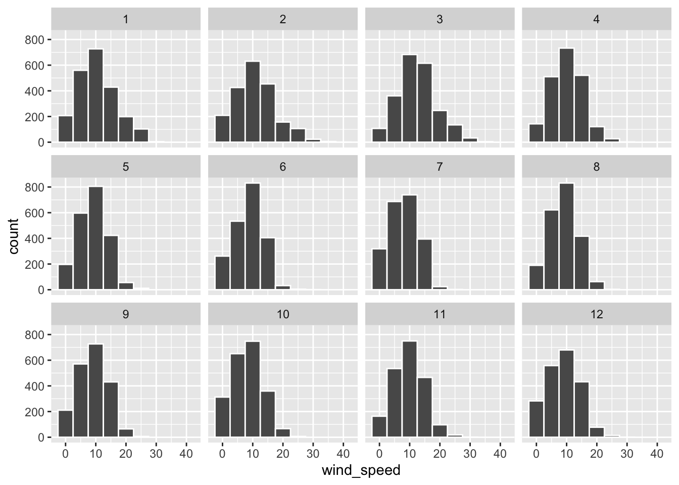
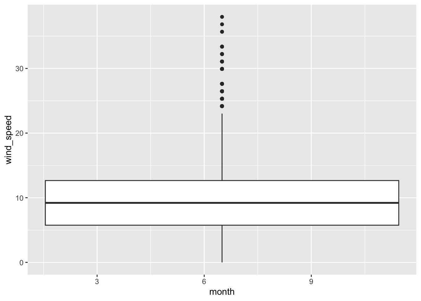
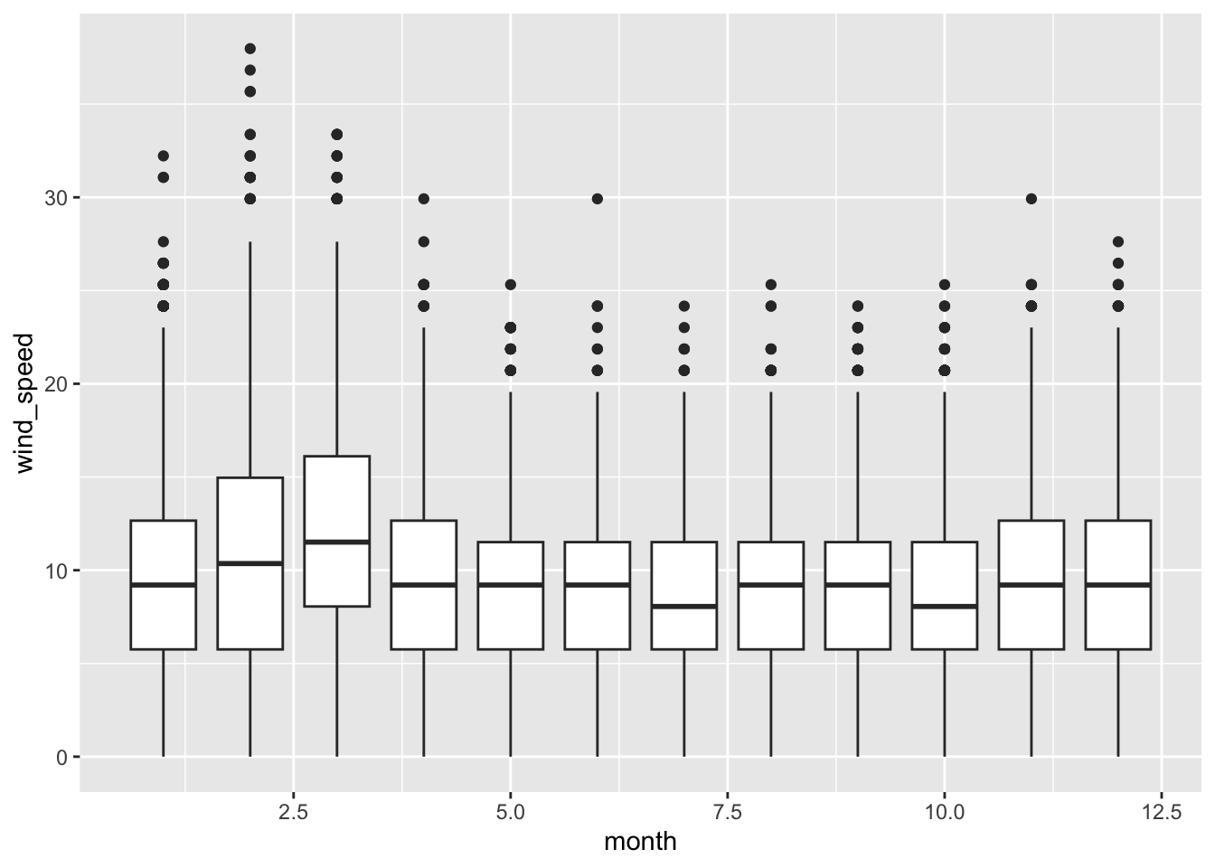
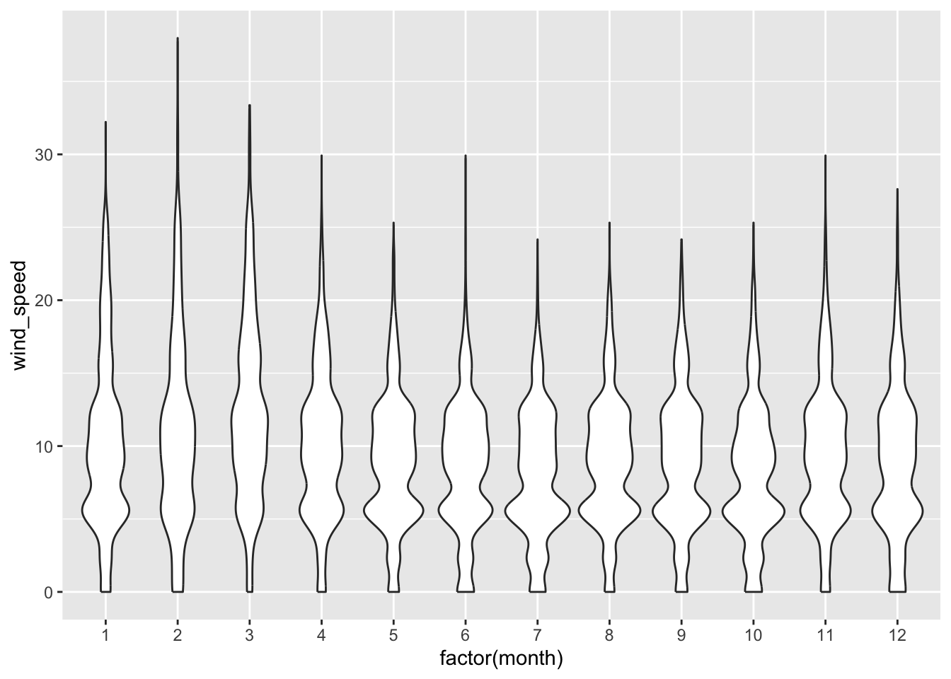
$ month      <int> 1, 1, 1, 1, 1, 1, 1, 1, 1, 1, 1, 1, 1, 1, 1, 1, 1, 1, 1, 1,…
$ day        <int> 1, 1, 1, 1, 1, 1, 1, 1, 1, 1, 1, 1, 1, 1, 1, 1, 1, 1, 1, 1,…
$ hour       <int> 0, 1, 2, 3, 4, 5, 6, 7, 8, 9, 10, 11, 12, 13, 14, 15, 16, 1…
$ temp       <dbl> 48.0, 48.2, 49.0, 49.0, 49.0, 48.0, 46.4, 46.0, 48.0, 47.0,…
$ dewp       <dbl> 48.0, 48.2, 49.0, 49.0, 49.0, 48.0, 46.4, 46.0, 48.0, 47.0,…
$ humid      <dbl> 100.00, 100.00, 100.00, 100.00, 100.00, 100.00, 100.00, 100…
$ wind_dir   <dbl> 0, 190, 190, 250, 170, 0, 250, 230, 260, 250, 240, 260, 260…
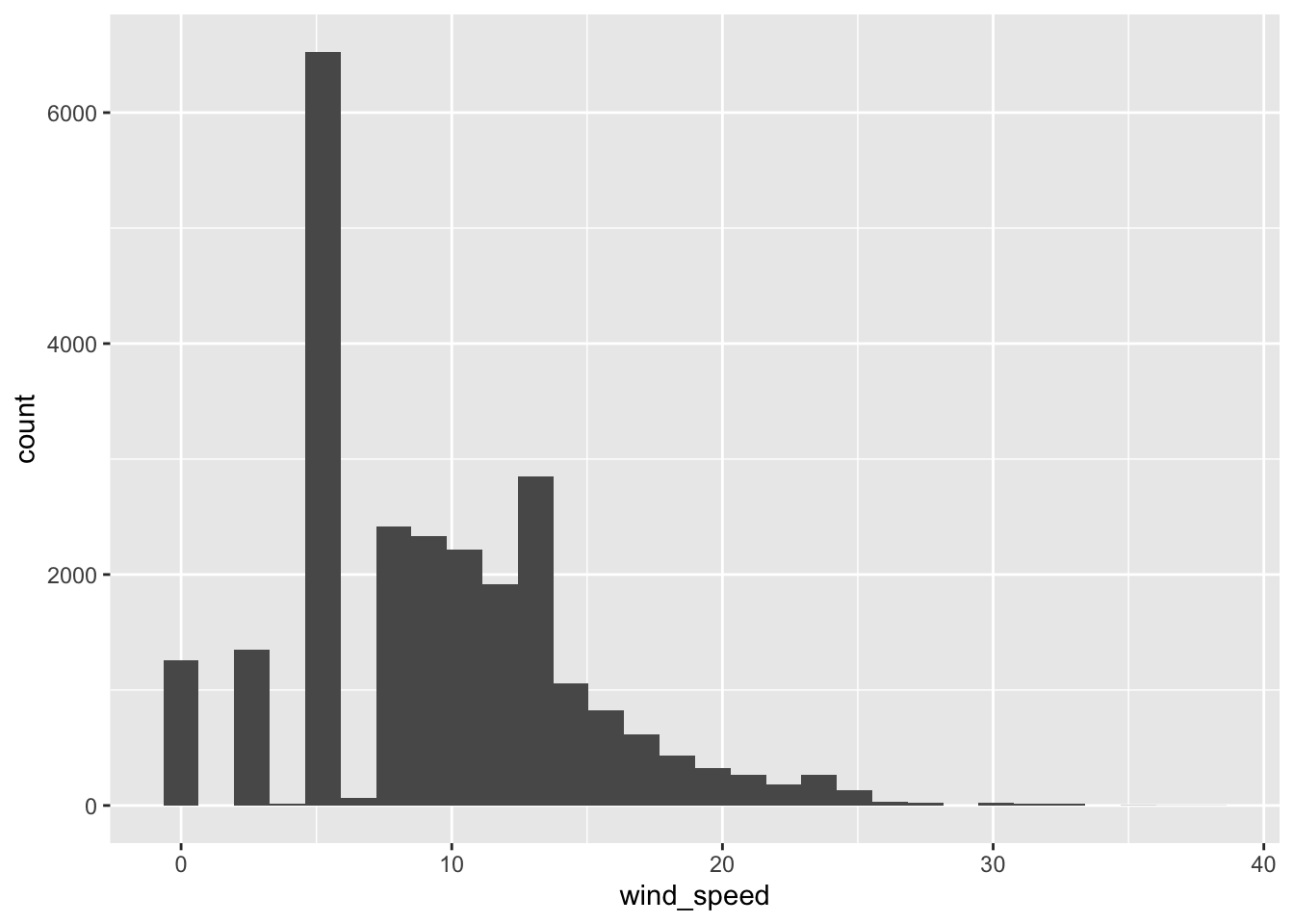
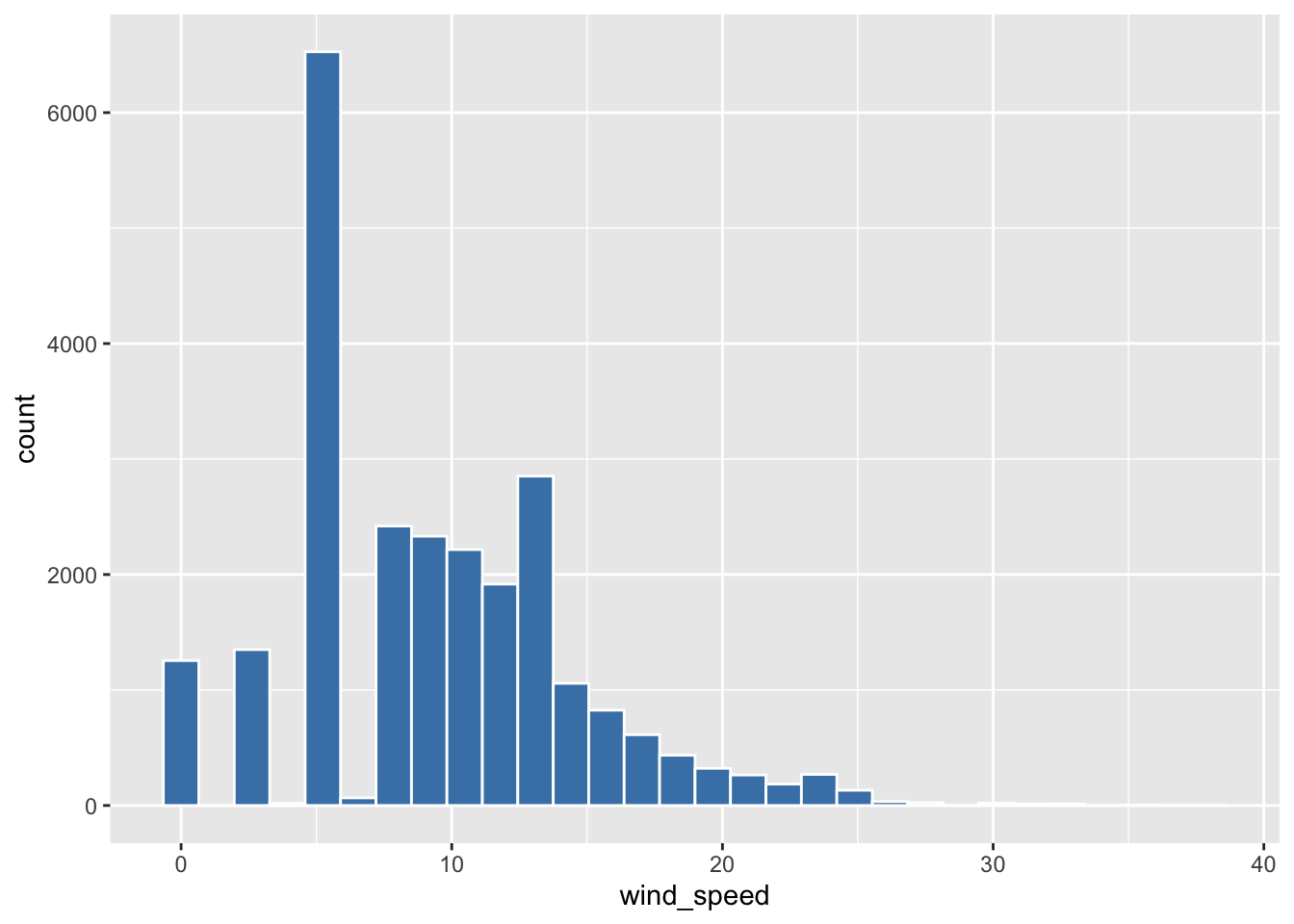
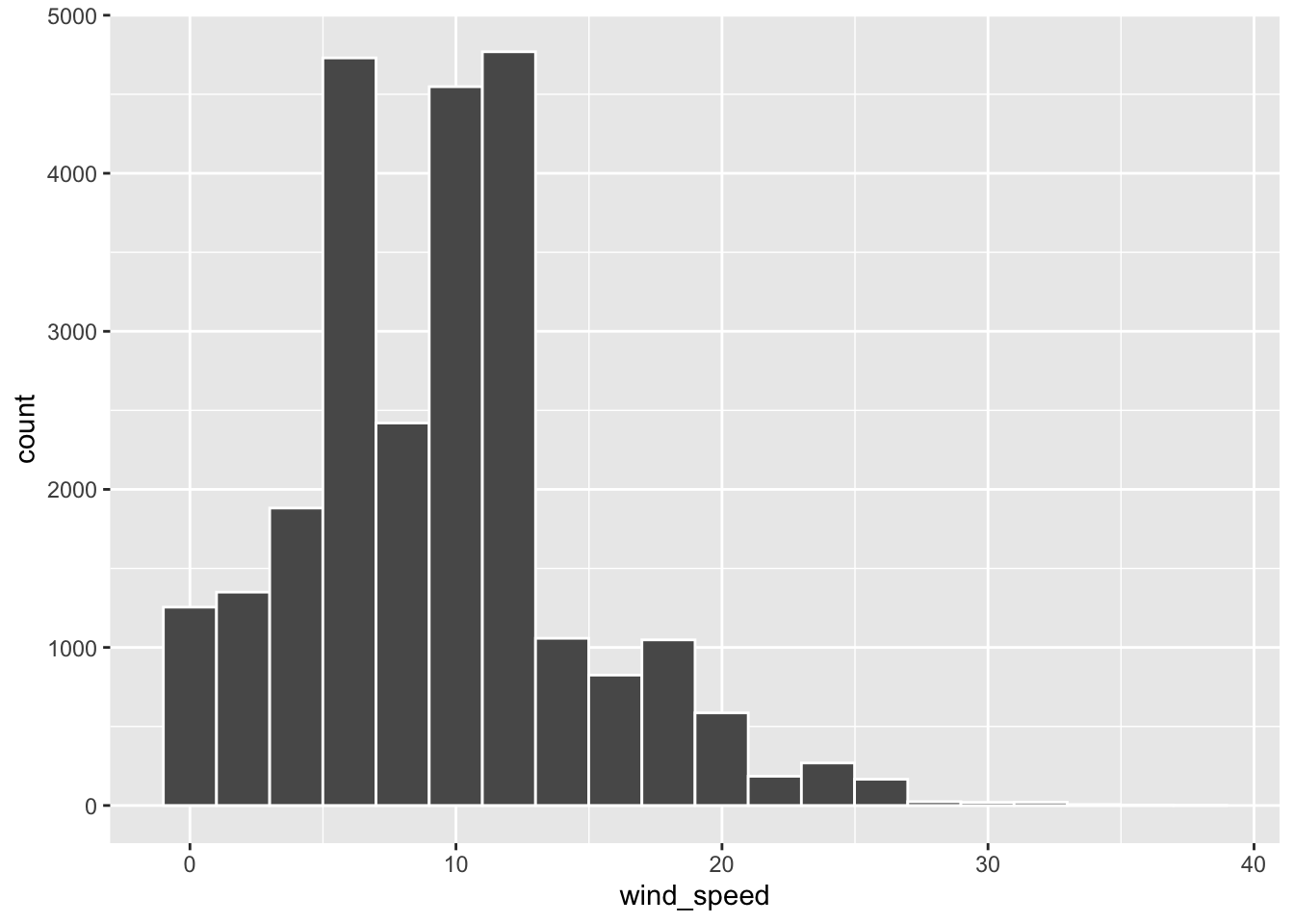
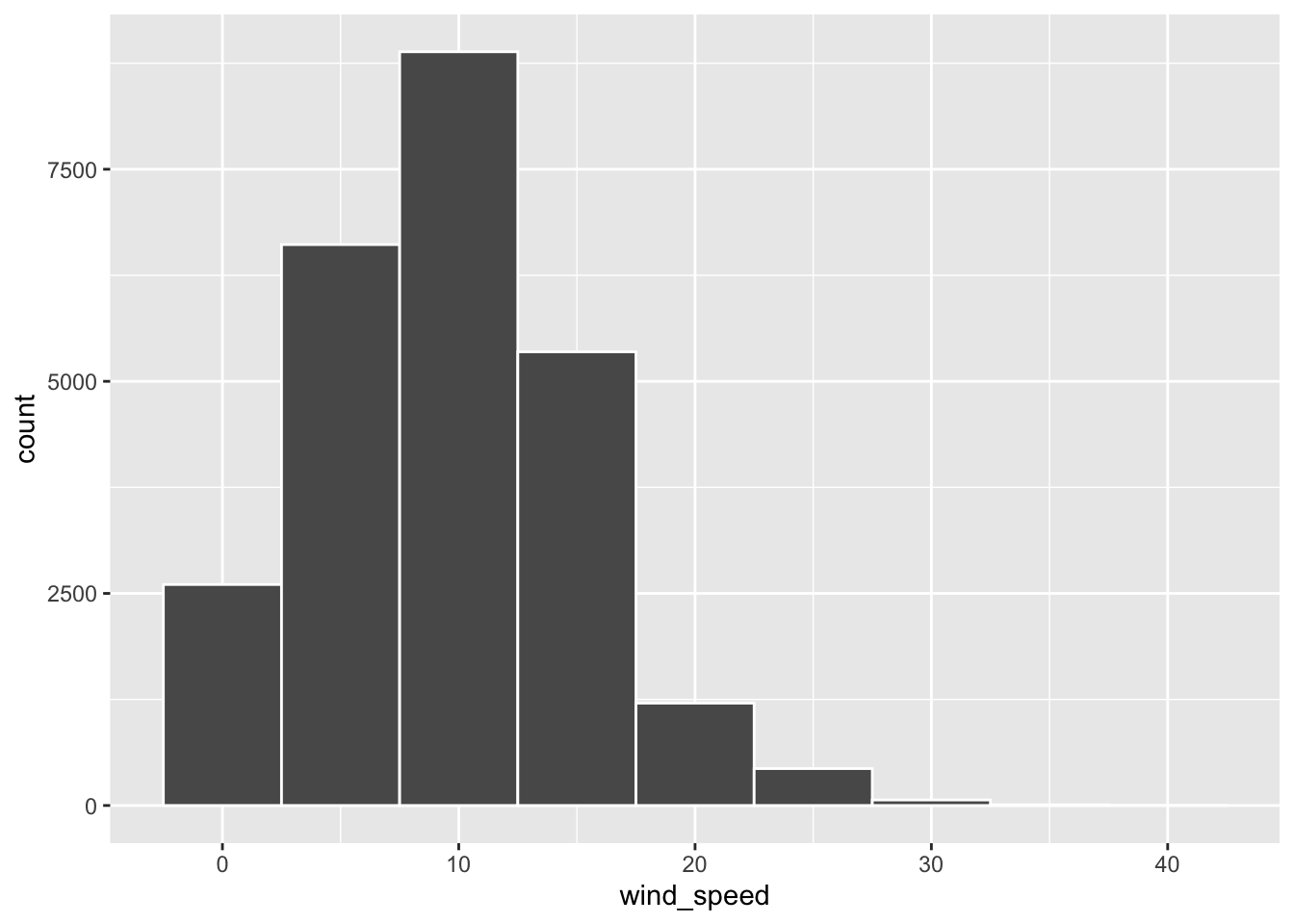
$ wind_speed <dbl> 0.00000, 4.60312, 5.75390, 5.75390, 8.05546, 0.00000, 9.206…
$ wind_gust  <dbl> 0.000000, 5.297178, 6.621473, 6.621473, 9.270062, 0.000000,…
$ precip     <dbl> 1e-02, 1e-02, 1e-04, 2e-02, 1e-04, 1e-04, 0e+00, 0e+00, 0e+…
$ pressure   <dbl> 1010.2, 1009.2, 1009.0, 1008.0, 1007.8, 1007.6, 1007.3, 100…
$ visib      <dbl> 0.25, 2.50, 0.25, 4.00, 0.75, 0.75, 0.24, 0.50, 8.00, 5.00,…
$ time_hour  <dttm> 2023-01-01 00:00:00, 2023-01-01 01:00:00, 2023-01-01 02:00…

ggplot(data = early_january_2023_weather, 
       mapping = aes(x = time_hour, y = wind_speed)) +
  geom_line()

Histograms

Shows the distribution of a variable.

ggplot(data = weather, mapping = aes(x = wind_speed)) +
  geom_histogram()

`stat_bin()` using `bins = 30`. Pick better value with `binwidth`.

Warning: Removed 1041 rows containing non-finite outside the scale range
(`stat_bin()`).

ggplot(data = weather, mapping = aes(x = wind_speed)) +
  geom_histogram(color = "white", fill = "steelblue")

`stat_bin()` using `bins = 30`. Pick better value with `binwidth`.

Warning: Removed 1041 rows containing non-finite outside the scale range
(`stat_bin()`).

adjusting bins

number of bins

ggplot(data = weather, mapping = aes(x = wind_speed)) +
  geom_histogram(bins = 20, color = "white")

Warning: Removed 1041 rows containing non-finite outside the scale range
(`stat_bin()`).

binwidth

ggplot(data = weather, mapping = aes(x = wind_speed)) +
  geom_histogram(binwidth = 5, color = "white")

Warning: Removed 1041 rows containing non-finite outside the scale range
(`stat_bin()`).

Facets

Dividing plots by subcategories in the data.

ggplot(data = weather, mapping = aes(x = wind_speed)) +
  geom_histogram(binwidth = 5, color = "white") +
  facet_wrap(~ month)

Warning: Removed 1041 rows containing non-finite outside the scale range
(`stat_bin()`).

Boxplots

Display the distribution of data and include five numbers to summarize the data:

minimum
first quartile (25th percentile)
median (2nd quartile, 50th percentile)
third quartile (75th percentile)
maximum
also shows the IQR (middle 50%)
- whiskers extend no more than 1.5 IQR units beyond 25th and 75 percentile.
- points beyond 1.5 IQR units may be considered outliers.

ggplot(data = weather, mapping = aes(x = month, y = wind_speed)) +
  geom_boxplot()

Warning: Continuous x aesthetic
ℹ did you forget `aes(group = ...)`?

Warning: Removed 1041 rows containing non-finite outside the scale range
(`stat_boxplot()`).

Note

Returns an invalid plot and a warning.

ggplot(data = weather, mapping = aes(x = month, y = wind_speed, group = month)) +
  geom_boxplot()

Warning: Removed 1041 rows containing non-finite outside the scale range
(`stat_boxplot()`).

represent months as factors and use geom(violin) for a more detailed plot.

ggplot(data = weather, mapping = aes(x = factor(month), y = wind_speed)) +
  geom_violin()

Warning: Removed 1041 rows containing non-finite outside the scale range
(`stat_ydensity()`).

Barplots

Simpler representation of the distribution known as frequencxies - depends on whether the items are counted or not.

fruits <- tibble(fruit = c("apple", "apple", "orange", "apple", "orange"))
fruits_counted <- tibble(
  fruit = c("apple", "orange"),
  number = c(3, 2))

ggplot(data = fruits, mapping = aes(x = fruit)) +
  geom_bar()

ggplot(data = fruits_counted, mapping = aes(x = fruit)) +
  geom_bar()

ggplot(data = fruits_counted, mapping = aes(x = fruit, y = number)) +
  geom_col()

when items are not counted, use geom_bar() with fruit mapped to the x aes
when items are counted, we add number to the y aes and use geom_col()

ggplot(flights,  aes(x = carrier)) +
  geom_bar()

geom_histogram() has bars that touch, but geom_bar() has bars with white space between

View(airlines)

Important

The best pie-chart is a bar-chart.

Stacked Barplot

ggplot(data = flights, mapping = aes(x = carrier, fill = origin)) +
  geom_bar()

Dodged Barplot

ggplot(data = flights, mapping = aes(x = carrier, fill = origin)) +
  geom_bar(position = "dodge") +
  scale_fill_viridis_d(option = "plasma")

Summary

Named graph	Shows	Geometric object	Notes
1	Scatterplot	Relationship between 2 numerical variables geom_point()
2	Linegraph	Relationship between 2 numerical variables geom_line()	Used when there is a sequential order to x-variable, e.g., time
3	Histogram	Distribution of 1 numerical variable geom_histogram()	Facetted histograms show the distribution of 1 numerical variable split by the values of another variable
4	Boxplot	Distribution of 1 numerical variable split by the values of another variable geom_boxplot()
5	Barplot	Distribution of 1 categorical variable geom_bar() when counts are not pre-counted, geom_col() when counts are pre-counted	Stacked, side-by-side, and faceted barplots show the joint distribution of 2 categorical variables